How AlphaGenome Models Gene Regulation: 2D Embeddings, Splicing, and the Race to Read Non-Coding DNA

Consider a single point mutation in the SMN1 gene. It sits at a splice donor site, two nucleotides from an exon boundary. A 1D sequence model scanning this region sees a local disruption: one base changed, one motif broken. What it cannot see is the downstream acceptor site 40 kilobases away that would normally pair with this donor. It also misses the branch point sequence buried deep in the intron and the exonic splicing enhancer three exons upstream that modulates inclusion of this cassette exon. That blind spot is not academic. An estimated one in three disease-associated variants disrupt RNA splicing ¹, causing conditions from spinal muscular atrophy to certain forms of cystic fibrosis ².

AlphaGenome, Google DeepMind's unified DNA sequence model published in Nature on January 28, 2026 ³, addresses this gap. It processes 1 million base pairs of DNA at single-nucleotide resolution while simultaneously predicting thousands of functional outputs across 11 modalities ⁴. But the real advance is architectural: AlphaGenome introduces two-dimensional pairwise embeddings alongside conventional 1D representations, giving it the vocabulary to reason about donor-acceptor splice site interactions directly. The result is state-of-the-art performance on 6 of 7 splicing benchmarks ⁵, surpassing specialized models like SpliceAI and Pangolin that were purpose-built for this exact task.

This post unpacks how AlphaGenome's architecture handles the inherently two-dimensional nature of splicing, why its multimodal training produces better splice predictions than single-task models, and what the benchmarks actually measure for clinical variant interpretation. If you build sequence-to-function models or work on variant interpretation pipelines, this is the engineering blueprint worth studying.

Two Approaches to Genomic AI

Before examining AlphaGenome's architecture, it helps to understand the split in genomic deep learning that shaped its design.

One camp builds self-supervised foundation models: train on raw DNA sequences, then fine-tune for downstream tasks. The Nucleotide Transformer uses masked language modeling across 2.5 billion parameters and 3,202 human genomes ⁶. HyenaDNA processes up to 1 million tokens at single-nucleotide resolution using sub-quadratic attention alternatives ⁷. Evo 2 scales to 40 billion parameters trained on 9.3 trillion base pairs from all domains of life ⁸. These models learn general sequence representations, but they require task-specific adaptation to predict functional outputs like gene expression or splicing.

The other camp builds supervised multi-task models: train directly on experimental functional genomics measurements. Enformer predicts gene expression and chromatin states from 196,608 bp of input at 128-bp resolution ⁹. Borzoi extends context to 524 kb but bins predictions at 32 bp ¹⁰. Both predict measurable quantities like RNA-seq coverage and ChIP-seq peaks. Both treat DNA as a one-dimensional signal.

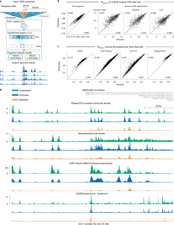Figure 1: Enformer, the predecessor to AlphaGenome, uses a convolutional trunk followed by transformer layers. It processes 196 kb of input at 128-bp resolution, a 5x improvement over prior methods but still limited for fine-grained splicing analysis. Source: Avsec et al., Nature Methods (2021), Figure 1.

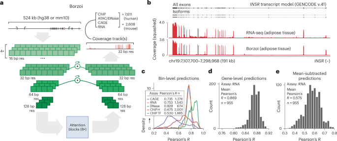Figure 2: Borzoi extends context to 500 kb with 32-bp resolution bins, directly predicting RNA-seq coverage. This was the strongest gene expression model before AlphaGenome. Source: Kelley, Nature Genetics (2024), Figure 1.

AlphaGenome sits at the supervised end of this spectrum but breaks from both predecessors in a critical way. It maintains single-base-pair resolution across a full megabase of context, and it introduces a 2D representation branch for pairwise genomic interactions. What splicing demands from a model explains why.

Why 1D Models Miss Splicing

Splicing is a pairing problem. A donor site (GT dinucleotide at the 5' end of an intron) must find and pair with an acceptor site (AG dinucleotide at the 3' end), sometimes tens of thousands of bases away. The strength of that pairing depends on the branch point sequence, polypyrimidine tract, exonic splicing enhancers and silencers, and chromatin structure. Representing these pairwise relationships in a purely 1D embedding is like trying to capture protein contact maps with just a sequence profile: you lose the relational structure.

Models like SpliceAI provide base-resolution predictions but accept only short input sequences of 10 kb or less, missing the influence of distal regulatory elements ¹¹. Enformer expanded the number of relevant enhancers seen by the model from 47% (at less than 20 kb) to 84% (at less than 100 kb) ¹², but its 128-bp bins cannot resolve individual splice sites. Borzoi improved gene expression prediction with 32-bp bins ¹⁰, but still smears the precise dinucleotides that define splice junctions. Neither model explicitly predicts which donor pairs with which acceptor.

The gap matters clinically. Variants disrupting mRNA splicing account for a sizable fraction of the pathogenic burden in many genetic disorders, but identifying splice-disruptive variants beyond the essential splice site dinucleotides remains difficult ¹³. A variant 50 kb upstream might reshape chromatin accessibility, alter transcription elongation kinetics, and shift the competition between alternative splice acceptors. Catching that requires both long-range context and the ability to reason about two positions jointly.

AlphaGenome's Architecture: The U-Net with Dual Embeddings

AlphaGenome takes a different approach. Rather than choosing between resolution and context, it uses a U-Net-inspired backbone to process input sequences into two types of representations: one-dimensional embeddings at 1-bp and 128-bp resolutions, and two-dimensional embeddings at 2,048-bp resolution ¹⁴.

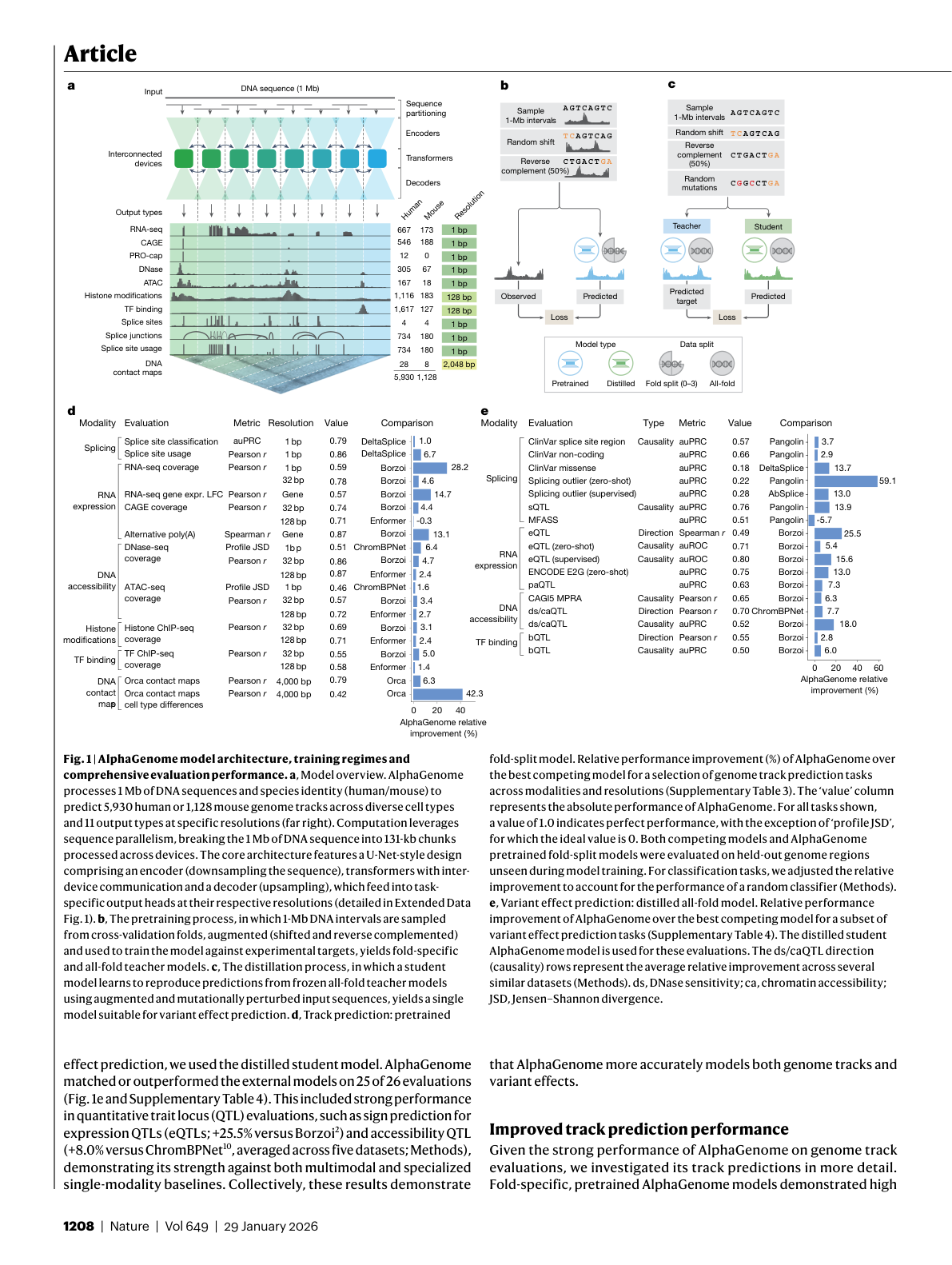Figure 3: AlphaGenome architecture overview showing the U-Net encoder-decoder, pre-training with 4-fold cross-validation, and distillation process. The model processes 1 Mb of DNA and outputs predictions across 11 modalities. Source: Avsec et al., Nature (2026), Figure 1.

The architecture breaks down into four stages ¹⁵:

• Seven convolutional downsampling stages detect motifs and progressively reduce sequence length while growing channel dimensions. These layers model local sequence patterns necessary for fine-grained predictions ¹⁶.
• Multi-head transformer layers enable long-range attention across the compressed representation, modeling coarser but longer-range dependencies such as enhancer-promoter interactions ¹⁶.
• 2D pairwise interaction blocks project the 1D representations into a square matrix of pairwise features. Each cell (i, j) encodes the relationship between genomic segments i and j, potentially capturing spatial proximity and splice site pairing.
• U-Net-style decoder with skip connections restores single-base resolution output, feeding into task-specific heads for each prediction modality.

Figure 4: Full architectural detail showing all block types, tensor shapes at each stage, the sequence-to-pair projection block, and the splice junction head. Source: Avsec et al., Nature (2026), Extended Data Fig. 1.

The 2D branch is not a bolt-on module. It shares parameters and gradients with the encoder that feeds the 1D output heads. When the model learns that a sequence motif affects splicing, that knowledge propagates through both branches. The design parallels AlphaFold's pairwise amino acid representations. Just as AlphaFold's pair track captures which residues sit close in 3D protein structure, AlphaGenome's 2D track captures which genomic positions interact in chromatin space and in donor-acceptor splice relationships.

This division of labor means the model can simultaneously recognize a GT dinucleotide at a splice donor (a local, 1-bp feature) and the regulatory context 500 kb away that influences whether that donor gets used. It processes 5x longer sequences at 128x higher resolution than Enformer ¹⁷. David Kelley, who built both Enformer and Borzoi, noted that this sequence length is "definitely one of those major engineering breakthroughs" ¹⁸.

import numpy as np
import jax.numpy as jnp
from alphagenome import dna_model

# Load the distilled student model from Kaggle weights.
# The student was distilled from 64 frozen teacher models,
# each trained with 4-fold cross-validation.
model = dna_model.create_from_kaggle("all_folds")

# Prepare a 1 Mb DNA input as one-hot encoding.
# A=[1,0,0,0], C=[0,1,0,0], G=[0,0,1,0], T=[0,0,0,1]
SEQ_LEN = 1_000_000
rng = np.random.default_rng(42)
random_indices = rng.integers(0, 4, size=SEQ_LEN)
one_hot = np.eye(4, dtype=np.float32)[random_indices]  # (1000000, 4)
input_seq = jnp.expand_dims(one_hot, axis=0)            # (1, 1000000, 4)

# Run model inference
outputs = model.predict(input_seq, species="human")

# Inspect output modalities and tensor shapes:
# 1D at 1-bp resolution -- splice site predictions
splice = outputs["splice_site"]
print(f"Splice sites:   {splice.shape}")   # (1, 1000000, N_splice_tracks)

# 1D at 128-bp resolution -- gene expression, accessibility
rna = outputs["rna_seq"]
print(f"RNA-seq:        {rna.shape}")      # (1, 7812, N_expression_tracks)

# 2D at 2048-bp resolution -- chromatin contact maps
contacts = outputs["contact_map"]
print(f"Contact maps:   {contacts.shape}") # (1, 488, 488, N_contact_tracks)

The Splice Junction Head: Predicting Donor-Acceptor Pairs

Most splicing models predict a per-position probability: is this base a splice donor or acceptor? AlphaGenome predicts that too, but it goes further. It predicts three distinct splicing quantities alongside direct RNA-seq coverage, providing a more comprehensive view of splice-related molecular consequences ¹⁹:

1. Splice site identity: binary classification of whether each position is a donor or acceptor (1-bp resolution, from the 1D branch).
2. Splice site usage (PSI): quantitative measure of how frequently each site is used across cell types and tissues, measured as percent-spliced-in values for donors (PSI5) and acceptors (PSI3). The same site may be used 80% of the time in liver but 20% in brain.
3. Splice junction coordinates and strength: a 2D prediction scoring the connection between a specific donor position and a specific acceptor position. This comes from the pairwise embedding branch.

The third output is what the 2D embeddings enable. At 2,048-bp resolution across a 1 Mb window, the model builds a matrix of roughly 488 x 488 pairwise positions. Each entry represents the predicted strength of a splice junction connecting a donor in segment i to an acceptor in segment j. The model scores all possible donor-acceptor pairings simultaneously, rather than relying on heuristics or sliding windows.

Consider what this means for variant interpretation. A mutation that weakens a canonical donor site produces a reduced donor probability in any 1D model. But a 1D model cannot tell you which downstream acceptor will now be favored. AlphaGenome's 2D junction prediction can show the redistribution of junction usage across alternative acceptors, revealing whether the variant causes exon skipping, intron retention, or activation of a cryptic splice site.

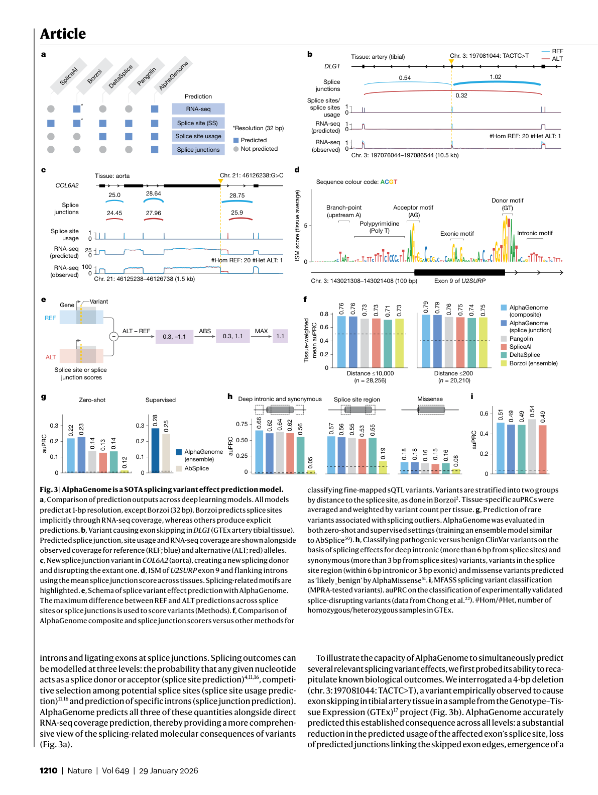Figure 5: Splicing variant effect prediction showing comparison across deep learning models, a DLG1 exon-skipping variant, and benchmark performance across splicing tasks. Source: Avsec et al., Nature (2026), Figure 3.

Splicing Benchmarks: What 6 of 7 Actually Means

AlphaGenome surpasses SpliceAI and Pangolin on 6 of 7 splicing tests ⁵. The interesting question is not just that it wins. It is how it wins, and on which tasks the gains matter most.

The splicing evaluations span three categories of clinical variants from ClinVar ²⁰:

• Deep intronic and synonymous variants: variants far from splice sites or within exons that do not change amino acids. AlphaGenome achieves auPRC 0.66 versus 0.64 by Pangolin.
• Splice region variants: variants near canonical splice sites. AlphaGenome achieves auPRC 0.57 versus 0.55 by Pangolin.
• Missense variants: coding variants that also disrupt splicing. AlphaGenome achieves auPRC 0.18 versus 0.16 by DeltaSplice and Pangolin.

For splice donor usage prediction, the model gains +12.7% (auPRC: 0.80 vs. 0.71) ²¹.

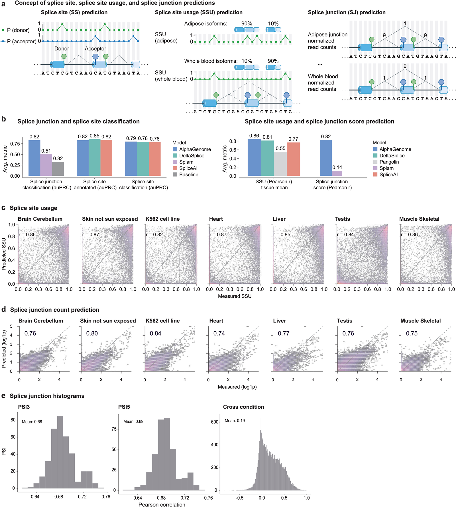Figure 6: Splicing prediction concepts and benchmark results. AlphaGenome leads across splice site identification, splice site usage, and splice junction prediction metrics. Source: Avsec et al., Nature (2026), Extended Data Fig. 2.

The deep intronic results are particularly telling. These variants sit far from the exon-intron boundary, well outside SpliceAI's 10 kb window. Detecting them requires both the 1 Mb context (to see distal splicing regulators) and the 2D pairwise representation (to model how those regulators alter donor-acceptor pairing). AlphaGenome also performed best on fine-mapped splicing QTL (sQTL) classification ²², which tests whether the model distinguishes truly causal splicing variants from nearby non-causal variants in linkage disequilibrium.

These margins may look small in absolute terms, but in a clinical pipeline processing thousands of variants of uncertain significance, they translate to meaningfully more correct classifications. The team developed a unified splicing variant scorer to systematically detect splice-disrupting variants ²³ across all three ClinVar categories.

Training: Sequence Parallelism, Distillation, and Why Multimodal Helps Splicing

AlphaGenome simultaneously predicts 5,930 human tracks and 1,128 mouse tracks spanning 11 modalities: RNA expression, CAGE, PRO-cap, splice sites, DNase, ATAC, histone marks, transcription factor binding, and Hi-C contact maps ²⁴. Training data comes from ENCODE, GTEx, 4D Nucleome, and FANTOM5 ²⁵.

Processing 1 million base pairs at single-nucleotide resolution demands serious engineering. Base-pair-resolution training on the full 1 Mb sequence runs via sequence parallelism across eight interconnected TPUv3 devices ²⁶. The input splits into 131 kb chunks processed across devices ²⁷, with inter-device communication during transformer layers.

The training follows two stages ²⁸:

Stage 1: Pre-training. Fold-specific models train using a 4-fold cross-validation scheme on 256 TPUv3 cores ²⁹. Training completes in approximately four hours, requiring half the compute budget of the original Enformer model ³⁰. Each run proceeds for 15,000 steps without early stopping ³¹.

Stage 2: Distillation. A single student model learns the ensemble average from 64 frozen teacher models on H100 GPUs ³². During distillation, 4% of the nucleotides in each input sequence are randomly mutated ³³, forcing the student to learn how the teacher ensemble responds to sequence changes rather than memorizing reference genome tracks. The distillation process runs for 250,000 steps over approximately 3 days ³⁴.

The random mutation during distillation is specifically important for splicing variant prediction. Without input perturbation, student model performance drops on splice-related tasks (sQTL causality: -0.01; splicing outlier: -0.015) ³⁵. The mutations teach the model to distinguish meaningful splice-disrupting changes from background variation.

A counterintuitive finding from the ablation studies: the fully multimodal model generally outperformed models trained on single modality groups ³⁶. You might expect a model trained only on splicing data to predict splicing best. That turns out to be wrong. Splicing does not happen in isolation. Chromatin accessibility determines whether the spliceosome can access a pre-mRNA. Histone modifications like H3K36me3 mark actively transcribed exons and influence splice site recognition. By training on all 11 modalities simultaneously, AlphaGenome learns the mechanistic connections between chromatin state, transcription, and splicing. Training at 1-bp resolution proved essential, consistently yielding the best results for fine-scale tasks like splicing (PSI5, PSI3) and accessibility (ATAC) ³⁷.

The distilled student model completes predictions in under one second on a single NVIDIA H100 GPU ³⁸, making large-scale variant screening practical.

import numpy as np
import jax.numpy as jnp
from alphagenome import dna_model

model = dna_model.create_from_kaggle("all_folds")

# Define the variant: a deep intronic G>T substitution
WINDOW = 1_000_000
variant_pos = 500_000  # center of the 1 Mb window

# Simulated reference sequence (in practice, load from a FASTA)
rng = np.random.default_rng(seed=123)
ref_indices = rng.integers(0, 4, size=WINDOW)

# Create REF and ALT one-hot encoded sequences
BASES = {"A": 0, "C": 1, "G": 2, "T": 3}
ref_indices[variant_pos] = BASES["G"]
alt_indices = ref_indices.copy()
alt_indices[variant_pos] = BASES["T"]

ref_input = jnp.expand_dims(np.eye(4, dtype=np.float32)[ref_indices], 0)
alt_input = jnp.expand_dims(np.eye(4, dtype=np.float32)[alt_indices], 0)

# Run inference on both alleles
ref_out = model.predict(ref_input, species="human")
alt_out = model.predict(alt_input, species="human")

# Extract PSI5 (donor usage) and PSI3 (acceptor usage) at 1-bp resolution
# Scoring method varies by modality:
#   Splice sites:  max absolute difference of probabilities
#   Gene expression: log-fold change
#   TF binding:      log2-ratio in a 501-bp window
ref_psi5 = ref_out["splice_site"][:, :, 0]
alt_psi5 = alt_out["splice_site"][:, :, 0]
ref_psi3 = ref_out["splice_site"][:, :, 1]
alt_psi3 = alt_out["splice_site"][:, :, 1]

# Compute splice disruption score
delta_psi5 = jnp.abs(alt_psi5 - ref_psi5)
delta_psi3 = jnp.abs(alt_psi3 - ref_psi3)
splice_delta = float(jnp.maximum(delta_psi5.max(), delta_psi3.max()))

# A quantile score > 1.0 means the effect exceeds 99% of common variants
QUANTILE_THRESHOLD = 1.0
print(f"Splice disruption score: {splice_delta:.4f}")
print(f"Exceeds 99th-percentile: {splice_delta > QUANTILE_THRESHOLD}")

From Benchmarks to Bedside: The Clinical Case for 2D Predictions

Beyond splicing, AlphaGenome's variant effect predictions span all 11 modalities. The model matched or exceeded the strongest available external models in 25 of 26 variant effect prediction evaluations ³⁹. Gains span gene expression (+14.7% over Borzoi) ⁴⁰, eQTL sign prediction (+25.5%) ⁴¹, and chromatin contact maps (+6.3% over Orca, with +42.3% for cell-type-specific differences) ⁴².

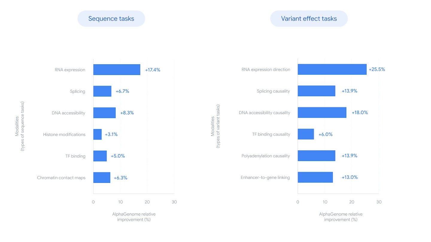Figure 7: Relative improvement over the best prior model for each task, across both sequence prediction and variant effect prediction. Splicing shows +6.7% on sequence tasks and +13.9% on variant causality. Source: Google DeepMind Blog.

For clinical genomics, two results stand out. First, at a score threshold yielding 90% sign prediction accuracy, AlphaGenome recovered over twice as many GTEx eQTLs (41%) as Borzoi (19%) ⁴³. For rare disease genetics, where most causal variants sit in non-coding regions, this recovery rate determines how many candidate variants a pipeline can flag for follow-up.

Second, the T-ALL (T-cell acute lymphoblastic leukemia) case study demonstrates the model's diagnostic potential. The team used AlphaGenome to investigate cancer-associated mutations at the TAL1 locus ⁴⁴. The model predicted that the mutations would activate TAL1 by introducing a MYB DNA binding motif ⁴⁵, with increased activating histone marks H3K27ac and H3K4me1 at the variant site consistent with experimentally observed neo-enhancer formation ⁴⁶. Years of wet-lab work had established this mechanism. AlphaGenome recovered it from sequence alone.

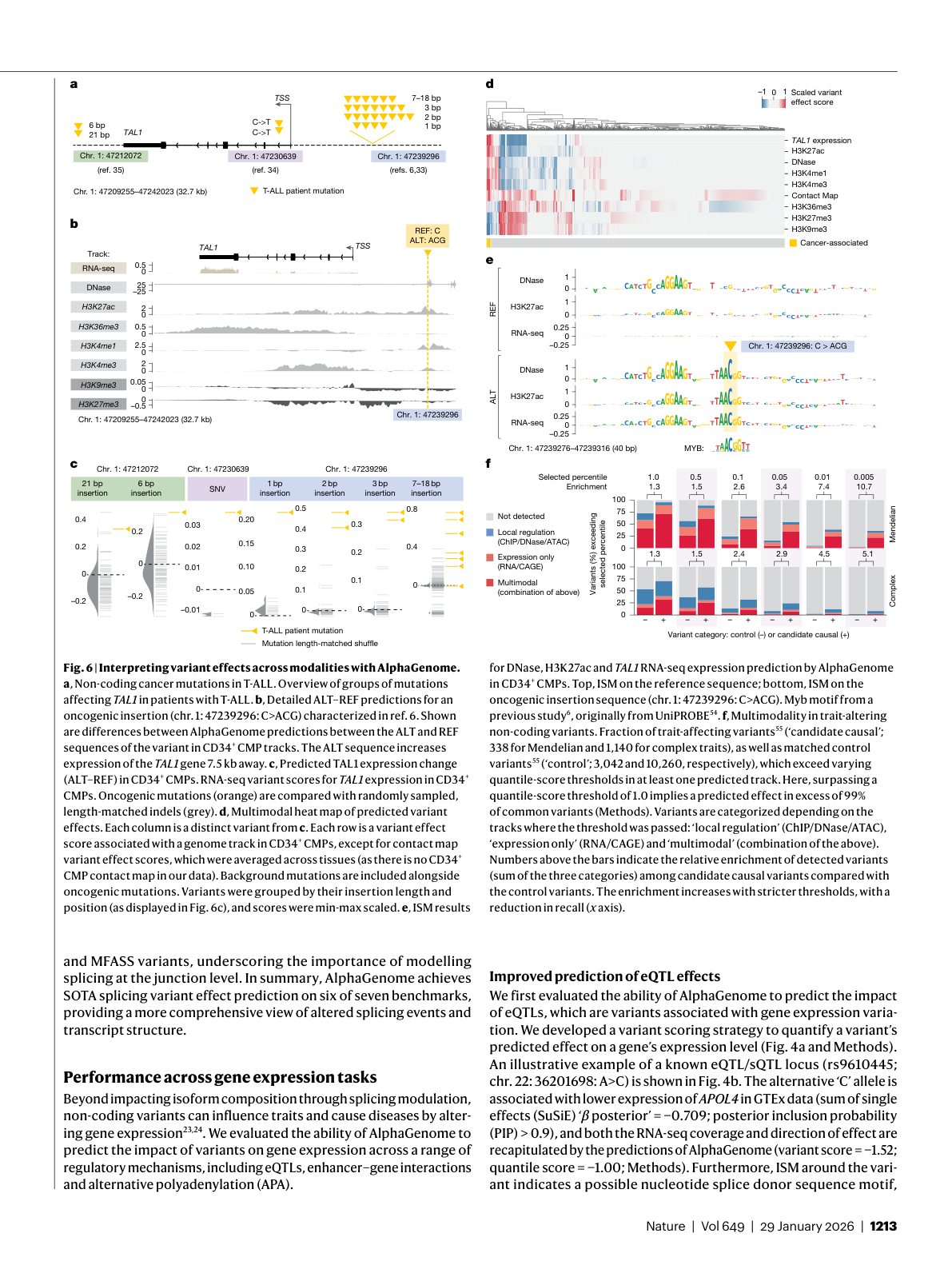Figure 8: AlphaGenome interprets non-coding T-ALL cancer mutations, showing ALT-REF predictions for the TAL1 locus across chromatin, expression, and binding modalities. Source: Avsec et al., Nature (2026), Figure 6.

Professor Marc Mansour of University College London described the clinical potential: "This tool will provide a crucial piece of the puzzle, allowing us to make better connections to understand diseases like cancer" ⁴⁷.

How AlphaGenome Compares to the Field

To place AlphaGenome's splicing capabilities in context:

Model	Context	Resolution	Splicing Support	Approach
SpliceAI	10 kb	1 bp	Splice sites only	Specialized CNN
Pangolin	10 kb	1 bp	Sites + usage	Specialized CNN
Enformer	196 kb	128 bp	Indirect (via bins)	Conv + Transformer
Borzoi	500 kb	32 bp	Indirect (via RNA-seq)	Conv + Transformer
Nucleotide Transformer	6 kb*	token-level	None (requires fine-tuning)	Masked LM
Evo 2	1 Mb	1 nt	None (generative)	Autoregressive
AlphaGenome	1 Mb	1 bp	Sites + usage + junctions	U-Net + Transformer + 2D

Nucleotide Transformer effective context varies by tokenization; typical window is approximately 6 kb ⁴⁸.

The supervised and self-supervised approaches are not competing so much as complementary. Self-supervised models like the Nucleotide Transformer learn general sequence representations that can be fine-tuned for various tasks. Supervised models like AlphaGenome learn task-specific predictions directly from experimental measurements. AlphaGenome can even complement generative DNA models by predicting functional properties of newly generated sequences ⁴⁹. As Dr. Robert Goldstone of the Francis Crick Institute described it, AlphaGenome is "a foundational, high-quality tool that turns the static code of the genome into a decipherable language" ⁵⁰.

Working with AlphaGenome

Google DeepMind open-sourced AlphaGenome on January 28, 2026 alongside the Nature publication ⁵¹. The JAX-based implementation is available on GitHub ⁵², with weights on Kaggle and Hugging Face ⁵³. Software code is licensed under Apache License 2.0, while model weights are for non-commercial use ⁵³.

Nearly 3,000 scientists across 160 countries currently submit approximately 1 million daily API requests ⁵⁴. The API suits smaller to medium-scale analyses (thousands of predictions) but exceeds practical limits for genome-wide scans requiring over 1 million predictions ⁵⁵. For large-scale work, the distilled student model runs locally on a single H100 GPU ⁵⁶.

import numpy as np
import jax.numpy as jnp
import pysam
from alphagenome import dna_model

MODEL = dna_model.create_from_kaggle("all_folds")
WINDOW = 1_000_000
BASE_TO_IDX = {"A": 0, "C": 1, "G": 2, "T": 3}

def score_splice_variant(chrom, pos, ref, alt, fasta_path):
    """Score a variant for splice disruption using AlphaGenome."""
    fasta = pysam.FastaFile(fasta_path)
    chrom_len = fasta.get_reference_length(chrom)
    half = WINDOW // 2
    start = pos - 1 - half  # convert to 0-based

    if start < 0 or start + WINDOW > chrom_len:
        raise ValueError(f"Variant at {chrom}:{pos} too close to edge")

    seq = fasta.fetch(chrom, start, start + WINDOW).upper()
    fasta.close()

    # Build REF and ALT one-hot tensors
    ref_idx = np.array([BASE_TO_IDX.get(b, 0) for b in seq])
    alt_idx = ref_idx.copy()
    assert seq[half] == ref, f"Mismatch: expected {ref}, got {seq[half]}"
    alt_idx[half] = BASE_TO_IDX[alt]

    ref_oh = jnp.array(np.eye(4, dtype=np.float32)[ref_idx])[None]
    alt_oh = jnp.array(np.eye(4, dtype=np.float32)[alt_idx])[None]

    # Run inference and extract PSI tracks
    ref_out = MODEL.predict(ref_oh, species="human")
    alt_out = MODEL.predict(alt_oh, species="human")

    deltas = np.abs(
        np.array(alt_out["splice_site"][0]) -
        np.array(ref_out["splice_site"][0])
    )
    splice_delta = float(deltas.max())

    # Report affected splice sites above threshold
    affected = []
    for col, label in enumerate(["PSI5", "PSI3"]):
        hits = np.where(deltas[:, col] > 0.05)[0]
        for h in hits:
            affected.append((label, start + int(h) + 1, float(deltas[h, col])))

    return {
        "splice_delta": splice_delta,
        "affected_sites": affected,
        "exceeds_quantile": splice_delta > 1.0,
    }

# Example: score a deep intronic HBB variant
result = score_splice_variant("chr11", 5_248_155, "G", "A", "/data/hg38.fa")
print(f"Splice score: {result['splice_delta']:.4f}")
print(f"Exceeds 99th percentile: {result['exceeds_quantile']}")

What Remains Hard

AlphaGenome's authors are candid about the remaining gaps.

Distance constraints. Accurately capturing the influence of distal regulatory elements beyond 100,000 base pairs remains a continuing objective ⁵⁷, despite the 1 Mb context. Some enhancer-promoter interactions span further.

Species coverage. The model covers only human and mouse genomes ⁵⁸. Extension to other organisms will require new training data.

Molecular predictions are not disease outcomes. AlphaGenome predicts molecular consequences of variants, but translating those to clinical phenotypes requires additional layers of biological interpretation ⁵⁹. As lead researcher Ziga Avsec put it: "Predicting how a disease manifests from the genome is an extremely hard problem, and this model is not able to magically predict that" ⁶⁰.

Exonic variant prediction is harder. Algorithms' concordance with experimental measurements is lower for exonic than intronic variants, underscoring the difficulty of identifying missense or synonymous splice-disruptive variants ⁶¹. AlphaGenome improves on this (missense auPRC: 0.18 vs. 0.16), but absolute performance on exonic splicing effects remains modest.

Personal genome prediction is unsolved. An independent evaluation from Mount Sinai found that despite improvements, AlphaGenome's performance still lags behind classic machine learning models trained directly on personal-level data ⁶². Professor Aldo Faisal of Imperial College London recommended treating results as promising rather than final pending independent verification ⁶³.

These limitations define the next set of problems. The 2D pairwise representation handles splicing better than any prior model, but it operates at 2,048-bp resolution in the pairwise dimension. Higher-resolution pairwise representations would capture finer-grained splice regulatory interactions. Extension beyond two species would test whether the learned representations transfer across evolutionary distance. And connecting molecular-level predictions to patient outcomes remains the gap between a powerful research tool and a clinical diagnostic.

The regulatory genome spans 98% of human DNA ⁶⁴. AlphaGenome is the first model that reads most of it at single-base resolution while reasoning about the pairwise interactions that give that sequence its meaning. What researchers and clinicians build on that foundation is the next chapter.

---

References

Footnotes

1. Wilks et al., "Benchmarking splice-disruptive variant predictors." Genome Biology (2023). ↩

2. Google DeepMind Blog (2025). ↩

3. Avsec, Z. et al. "Advancing regulatory variant effect prediction with AlphaGenome." Nature (2026). DOI: 10.1038/s41586-025-10014-0 ↩

4. Avsec et al., Nature (2026). ↩

5. Avsec et al., Nature (2026) summary. ↩ ↩²

6. Dalla-Torre, H. et al. "The Nucleotide Transformer." Nature Methods (2024). DOI: 10.1038/s41592-024-02523-z ↩

7. Nguyen, E. et al. "HyenaDNA." NeurIPS (2023). ↩

8. Arc Institute. "Evo 2." bioRxiv (2025). ↩

9. Avsec, Z. et al. "Effective gene expression prediction from sequence." Nature Methods (2021). DOI: 10.1038/s41592-021-01252-x ↩

10. Kelley, D. "Predicting RNA-seq coverage from DNA sequence." Nature Genetics (2024). DOI: 10.1038/s41588-024-02053-6 ↩ ↩²

11. Avsec et al., Nature (2026). ↩

12. Avsec et al., Nature Methods (2021). ↩

13. Wilks et al., Genome Biology (2023). ↩

14. Avsec et al., Nature (2026). ↩

15. Avsec et al., Nature (2026) and BinaryVerse AI summary. ↩

16. Avsec et al., Nature (2026). ↩ ↩²

17. Derived from Avsec et al., Nature Methods (2021) and Nature (2026). ↩

18. David Kelley, Calico Life Sciences. Quoted in Scientific American (2025). ↩

19. Avsec et al., Nature (2026). ↩

20. Avsec et al., Nature (2026). ClinVar benchmarks. ↩

21. Avsec et al., Nature (2026) summary. ↩

22. Avsec et al., Nature (2026). ↩

23. Avsec et al., Nature (2026). ↩

24. BinaryVerse AI summary. ↩

25. Google DeepMind Blog (2025). ↩

26. Avsec et al., Nature (2026). ↩

27. Avsec et al., bioRxiv (2025). ↩

28. Avsec et al., Nature (2026). ↩

29. Avsec et al., Nature (2026) summary. ↩

30. Google DeepMind Blog (2025). ↩

31. Avsec et al., bioRxiv (2025). ↩

32. BinaryVerse AI summary. ↩

33. Avsec et al., bioRxiv (2025). ↩

34. Avsec et al., bioRxiv (2025). ↩

35. Avsec et al., Nature (2026). ↩

36. Avsec et al., Nature (2026). ↩

37. Avsec et al., Nature (2026). ↩

38. Avsec et al., Nature (2026) summary. ↩

39. Avsec et al., Nature (2026). ↩

40. Avsec et al., Nature (2026) summary. ↩

41. Avsec et al., Nature (2026). ↩

42. Avsec et al., Nature (2026) summary. ↩

43. Avsec et al., Nature (2026). ↩

44. Google DeepMind Blog (2025). ↩

45. Google DeepMind Blog (2025). ↩

46. Avsec et al., Nature (2026). ↩

47. Professor Marc Mansour, UCL. Google DeepMind Blog (2025). ↩

48. Dalla-Torre et al., Nature Methods (2024). ↩

49. Avsec et al., Nature (2026). ↩

50. Dr. Robert Goldstone, Francis Crick Institute. Chemistry World (2026). ↩

51. Avsec et al., Nature (2026) summary. ↩

52. GitHub: https://github.com/google-deepmind/alphagenome_research ↩

53. SiliconANGLE (2026). ↩ ↩²

54. rewire.it (2025). ↩

55. AlphaGenome Documentation. ↩

56. STAT News (2026). ↩

57. Avsec et al., Nature (2026). ↩

58. Avsec et al., Nature (2026). ↩

59. Avsec et al., Nature (2026). ↩

60. Ziga Avsec, Scientific American (2025). ↩

61. Wilks et al., Genome Biology (2023). ↩

62. Shen, L. et al. Mount Sinai, bioRxiv (2025). DOI: 10.1101/2025.08.05.668750 ↩

63. Professor Aldo Faisal, Imperial College London. Science Media Centre (2026). ↩

64. Google DeepMind Blog (2025). ↩