A Protein Embedding Is Not an Explanation: Protein Language Models in 2026
Give one enzyme sequence to a protein language model and you can get at least three plausible answers. One API returns an matrix, one vector per residue. Another pools that matrix into a single -dimensional vector. A third scores the substitution glycine to aspartate from token probabilities. The checkpoint may be identical. The experimental artifacts are not.
That distinction matters if a lab has 300 measured substitutions, a separate pool of 10,000 unmeasured candidates and room for 96 in the next assay. A residue vector can feed a site-level predictor. A protein vector can feed a whole-sequence regressor. A zero-shot score can rank candidates without seeing those 300 labels. Different heads and splits can make any of the three look best.
Part 1, A FASTA File Is Not a Specification, treated a predicted structure as the output of a model, data path and run protocol. Part 2 of the six-part Foundation Models in Biology series moves upstream from the folding head. The question is not whether a model has “learned biology”. It is: which representation, extraction recipe and evaluation design support the claim we need to make?
Choose the claim before the tensor
For our enzyme, “predict mutation effect” is still underspecified. Are we ranking substitutions at positions already measured, unseen positions in the same wild type, or variants of a distant homologue? A model can succeed at the first and fail at the third without contradiction.
The output should follow that claim. Benchmarks such as TAPE distinguish residue, pair and protein-level tasks because their outputs and heads differ. In practice, four useful artifacts recur:
| Output | Mathematical object | Useful for | Does not establish |
|---|---|---|---|
| Residue representation | from layer | Secondary structure, sites, disorder, residue effects | A fixed representation of the whole protein |
| Protein representation | Function, localization, retrieval, one value per sequence | Which residues caused the result | |
| Zero-shot mutation score | Scalar from token log probabilities | Ranking substitutions without assay-label training | Calibration to the assay or a causal fitness effect |
| Structure-conditioned sequence distribution | Residue probabilities given a backbone or structural tokens | Inverse folding and sequence proposal | Experimental folding or function |
The first two are hidden states. The third comes from logits. The fourth reverses the direction of the problem. This pipeline makes the fork explicit.

Figure 1. Original synthesis of the sequence-to-artifact pipeline. The tensor and token-handling branches follow the documented extraction paths in the ProtT5 model card and ESMC-6B model card; the probability branch follows the zero-shot protocol in Meier et al.; the adaptation and head branches follow the transfer strategies compared in Bikias, Stamkopoulos and Reddy.
“We used ESM embeddings” is not a method. It omits almost every box in that diagram.
The objective and corpus decide what is cheap to recover
Widely used sequence encoders learn by repairing corrupted protein text. The foundational ESM work used masked-token prediction, and its authors showed that linear projections could recover secondary-structure and contact signal from hidden states (Rives et al., 2021). That supports a bounded statement: the states encode probe-accessible structural information. It does not supply a mechanism of catalysis.
ProtT5 changes both the architecture and corruption recipe. The live ProtT5-XL-UniRef50 card describes a roughly 3-billion-parameter T5-derived encoder-decoder trained with BART-like denoising and 15% masking on 45 million UniRef50 sequences. Inputs are uppercase, space-separated amino-acid tokens; U, Z, O and B become X. The documented pretraining pipeline truncated or padded sequences to 512 tokens (ProtTrans paper; model card, retrieved 28 August 2026). That 512-token training recipe is not a documented universal inference ceiling. Replacing selenocysteine with an unknown token or cutting a domain boundary changes the model input before a classifier sees it.
ProteinBERT is a useful counterexample to the idea that every protein vector is a mean over transformer tokens. Its roughly 16-million-parameter architecture jointly reconstructs sequence and Gene Ontology annotations while maintaining local residue states and a separate global state (Brandes et al., 2022). The GO objective is designed to privilege annotation-related signal. Whether that helps a target function is an empirical question, and annotation provenance becomes part of the pretraining audit.
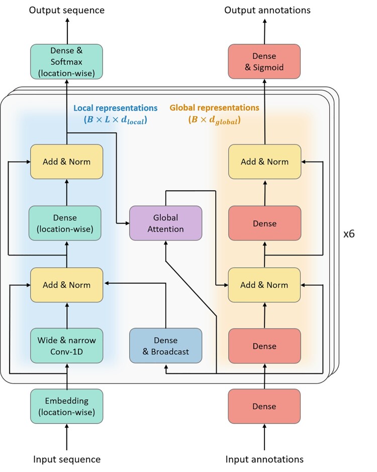
Figure 2. ProteinBERT explicitly maintains local residue states and a global protein state, with information moving between them. Source: Brandes et al., “ProteinBERT: a universal deep-learning model of protein sequence and function”, Fig. 1, CC BY 4.0. Unmodified.
Corpus construction applies another pressure. A study of more than 300 masked and causal protein models reported diminishing returns for causal models and overfitting when a masked model repeatedly saw a finite UniRef corpus. Adding metagenomic diversity changed the observed scaling frontier (Cheng et al., 2024). These are author-reported results under that training program, not a rule that one objective always wins. They do show why parameter count cannot summarize the data intervention.
The embedding is a recipe, not a checkpoint name
Even after choosing a checkpoint, the representation is not fixed. A sequence of retained tokens produces one matrix per layer. Useful transfer signal may appear before the final layer. Across 370 transfer experiments involving ESM and CARP, the largest gains on several tasks appeared in early layers and often plateaued, with task-specific exceptions (Li et al., 2024). PLMFit also reported task and adaptation sensitivity when varying the fraction of layers used across more than 3,000 configurations (Bikias et al., 2025).
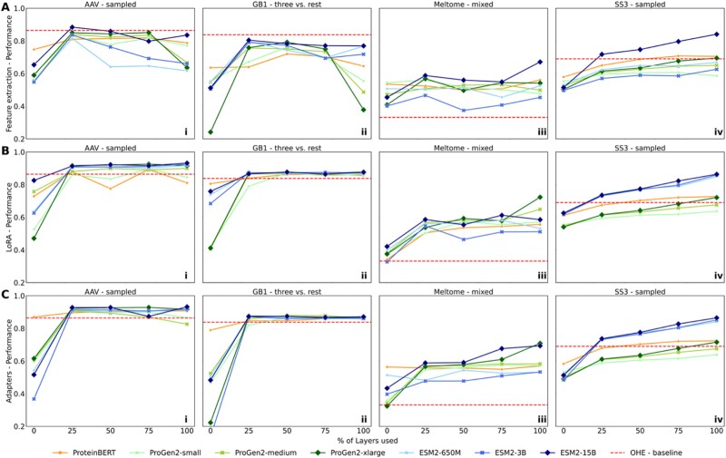
Figure 3. Useful depth varies across tasks, checkpoints and transfer strategies in the PLMFit experiments. Source: Bikias, Stamkopoulos and Reddy, “PLMFit: benchmarking transfer learning with protein language models for protein engineering”, Fig. 3, CC BY 4.0. Unmodified. These are author-reported, protocol-specific results, not a cross-model ranking.
“Use the last layer” is therefore a default to test. Cache two or three prespecified layers, then compare them with the same split, pooler, head, optimizer budget and seeds. If the preferred layer changes with the head, report the interaction.
Pooling is another model. Mean pooling weights every retained residue equally and removes explicit position at the aggregation step. A learned set function adds supervised capacity. NaderiAlizadeh and Singh made the separation clean by freezing the language model and training a sliced-Wasserstein aggregation function on four property-prediction protocols (NaderiAlizadeh and Singh, 2025).
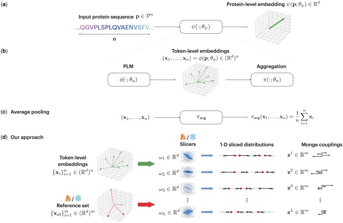
Figure 4. Residue vectors can be averaged or mapped against a learned reference distribution. The latter makes aggregation trainable. Source: NaderiAlizadeh and Singh, “Aggregating residue-level protein language model embeddings with optimal transport”, Fig. 1, CC BY 4.0. Unmodified.
Their reported comparisons are evidence about a frozen PLM plus a trained pooler. They do not prove that one raw checkpoint contains more biological information.
Record the exact checkpoint revision, tokenizer and normalization, context or windowing rule, selected layer, special-token handling, pooling, dtype and library version. Treat numerical precision as a sensitivity test, not a presumed effect: rerun a representative subset at the reference precision and check whether close rankings or neighbours change. A stated 2,048-token context means the model accepts that input length. It does not prove reliable long-range biology at residue 1,900.
Adaptation has two axes
For a masked model, a common single-substitution score compares mutant and wild-type log probabilities under the same masked context (Meier et al., 2021):
No assay-trained head is fitted and the pretrained weights do not change. That is what zero-shot means here. It does not mean the protein or its homologues were absent from pretraining. ESM-1v's developers evaluated 41 deep-mutational-scanning assays and found large assay variation; in their paired t-test over per-assay absolute Spearman correlations, ESM-1v and DeepSequence were not statistically distinguishable (Meier et al., 2021).
Once labels enter, separate two axes:
| Axis | Choices | What changes |
|---|---|---|
| Backbone state | Fixed likelihood rule; frozen checkpoint; LoRA; bottleneck adapters; full fine-tuning | From no assay-specific representation learning to low-rank updates, inserted modules or changes throughout the checkpoint |
| Downstream capacity | No head; linear probe; nonlinear predictor; learned pooler | From direct scoring to increasingly capable supervised mappings over the representation |
A probe is not a separate kind of hidden state. A linear probe is a deliberately weak head trained on frozen features. A nonlinear head is still a frozen-backbone experiment, but it can learn enough task structure to conceal differences between representations. LoRA learns low-rank weight updates, while bottleneck adapters insert trainable modules (Bikias et al., 2025).
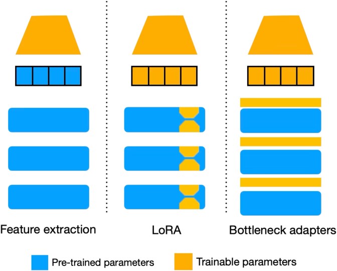
Figure 5. Frozen features, LoRA and bottleneck adapters place trainable parameters in different parts of the computation graph. Source: Bikias, Stamkopoulos and Reddy, “PLMFit”, Fig. 2, CC BY 4.0. Unmodified.
A peer-reviewed cross-model study of ESM-2, ProtT5 and Ankh reported that supervised adaptation usually helped across its eight tasks, although five of 64 model-task combinations worsened. Its authors also reported LoRA training up to 4.5 times faster on the largest tested setup, with mixed precision, length-1,024 inputs and a specific memory-efficient stack (Schmirler, Heinzinger and Rost, 2024). That is a protocol boundary, not a universal speed or memory claim.
For the 300 labelled enzyme substitutions, start with a zero-shot score and one-hot ridge regression, then use one fixed linear head on frozen states. Add a nonlinear head, LoRA or full tuning only if the simpler configuration fails under the same split and the expected gain justifies another experiment.
ESM is an ecosystem, not a version ladder
The archived Meta repository spans several branches: ESM-1b and ESM-2 for sequence representations, ESM-1v for variant scoring, MSA Transformer for aligned families, ESM-IF1 for inverse folding and the original ESMFold structure system (Meta ESM repository). MSA Transformer consumes an alignment and alternates attention over its rows and columns, so database search, alignment construction, depth and sampling belong to the input protocol (Rao et al., 2021). The original ESMFold combines ESM-2 representations with a trained folding architecture (Lin et al., 2023). Neither is simply “a newer embedding”.
For this article, current Biohub artifacts occupy three relevant roles. ESMC supplies sequence representations. ESMFold2 combines ESMC-6B embeddings with a diffusion-based folding architecture. ESM3 is a separate multimodal generative model over discrete sequence, structure and function tracks (Biohub repository; ESM3 documentation). The ESM3 developers report that their largest training run used 98 billion parameters, 2.78 billion proteins and 1.07 × 10^24 FLOPs (Hayes et al., 2025). That scale belongs to a multimodal generation claim. It is not evidence that ESM3 is the right frozen encoder for our assay.
The practical comparison is conditional:
| Exact artifact | Scale and training corpus | Context, architecture and input | Access and terms, checked 28 Aug 2026 | Compute evidence and plausible first fit |
|---|---|---|---|---|
| Biohub ESMC-6B | 6B parameters, 80 layers; UniRef, MGnify and JGI clustered at 70% identity | Transformer, single sequence; 512-token then 2,048-token training stages; all-layer states available | Local Hugging Face or hosted Biohub; repository licence is MIT, while the ESMC-6B card metadata lists mit and other and links a third-party notice. Re-check the checkpoint and dependencies |
Card reports 2.37 × 10^23 training FLOPs. Measure inference at target lengths. Strong first candidate for residue or protein representations (model card) |
| Rostlab ProtT5-XL-UniRef50 | About 3B parameters; 45M UniRef50 sequences | T5-derived encoder-decoder; BART-like denoising; documented 512-token pretraining preprocessing, not an established inference ceiling, and residue normalization | Hugging Face model card; the cited card does not establish terms for all code, weights or downstream uses, so verify the exact artifact | The original pretraining setup does not predict local inference cost. Measure target-length execution. Useful when its documented residue and mean-pooling path fits the task (model card) |
| OpenProtein.AI PoET-2 | 182M parameters; 62M homolog sets built from UniRef50 v2304 | Hierarchical retrieval context, optional structure, causal and bidirectional decoders; the cited paper and repository do not document one universal single-sequence context limit | Local execution from the official repository; source code excluding weights is Apache 2.0 subject to listed third-party component terms; model weights use the PoET Non-Commercial License Agreement | End-to-end cost includes search and prompt construction. Consider when homolog retrieval is available at deployment, not as a drop-in lone-sequence encoder (paper; repository) |
This is not a ranking. It exposes missing facts as decisions. Pretraining FLOPs do not tell you peak inference memory. Parameter count does not include MSA search, structure prediction or retrieval. Run each survivor on the target hardware, at the actual length distribution, and record peak memory, latency, throughput, truncation and failures.
Licensing needs the same precision. The current Biohub repository and named ESM3 documentation point to MIT terms, and the archived Meta source repository separately contains an MIT licence (Biohub licence; Meta repository). Those facts do not automatically cover every historical weight, hosted service, training record, paper figure or generated output. Record code, weights, data, service and output rights independently, with the retrieval date.
Structural signal, inverse folding and function need different tests
Sequence-only hidden states can support contact or secondary-structure probes without being coordinates, a folding system or an explanation. Architecture also changes resource scaling. In the CARP authors' hardware experiment, their 640-million-parameter dilated-convolution model scaled linearly with sequence length while ESM-1b's full attention scaled quadratically (Yang, Fusi and Lu, 2023). That is a reason to test CARP on a long-sequence workload, not a cross-task accuracy claim.
SaProt pairs amino-acid identity with Foldseek 3Di structure tokens, so the source and quality of the experimental or predicted structure become part of inference (Su et al., 2024). ProstT5 translates between amino-acid and 3Di strings (Heinzinger et al., 2024). ESM-IF1 instead starts from backbone coordinates; its developers augmented training with 12 million AlphaFold2-predicted structures and evaluated on topology-held-out backbones (Hsu et al., 2022). Native-sequence recovery under that protocol is not experimental proof that a proposal folds or functions.
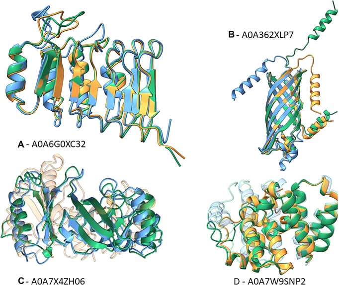
Figure 6. Four manually selected ProstT5 inverse-folding examples compare target and predicted structures. Source: Heinzinger et al., “Bilingual language model for protein sequence and structure”, Fig. 4, CC BY 4.0. Unmodified. Because the authors selected these examples manually, they are qualitative illustrations, not a benchmark or wet-lab validation.
Function prediction has its own complete pipeline. Here is the evaluation protocol I would use. Start with a pooled protein vector for whole-protein labels, or residue states for localized labels. Fit a hierarchical multi-label head, preserve ontology relations and choose thresholds on validation data. Then compare against BLAST, HMM and annotation-transfer baselines so the experiment measures value beyond family similarity.
Evaluate on family-held-out proteins and, where the claim is “annotate newly characterized proteins”, on later annotations. CAFA4 used such a prospective annotation boundary, evaluating submitted predictions after experimental annotations accumulated; its report covered 148 methods from 70 groups over five years and found weaker results for partially known proteins (Ramola et al., 2026). The output belongs to the representation, head, ontology snapshot, thresholds and split together.
The head may have won
A checkpoint does not generate an F-score by itself. If one system uses a linear probe and another uses a large multilayer head, the comparison is between systems. The head may have won.
To compare representation quality, hold the labelled data, split, preprocessing, layer-selection budget, pooling rule, head architecture, optimizer search, seeds and metric fixed. Change one checkpoint. To choose the best deployable pipeline, let each candidate use its best validated recipe and call the result a system comparison. Both experiments are useful. They answer different questions.
The same separation applies to folding heads, learned poolers and structure-token preprocessing. A downstream result can be excellent without showing that an untouched embedding is intrinsically superior.
A biologically honest split has two boundaries
Only the 300 measured enzyme substitutions belong in the supervised split. The 10,000 candidates are unmeasured deployment inputs, not rows to scatter across train and test. If the next assay targets unseen positions in the same enzyme, group the 300 measurements by position and hold positions out. If deployment changes the wild type or family, hold out those backbones or homology clusters instead.
Random sequence or variant splits can place close homologues, the same wild type and repeated positions on both sides. FLIP introduced low-resource and extrapolative protein-engineering splits because protein sequences are not independent, identically distributed rows (Dallago et al., 2021). Under the developer-reported FLIP2 protocols, ridge regression on one-hot sequence representations often matched or beat fine-tuned protein language models on harder deployment-shaped splits (Didi et al., 2026). Keep a humiliatingly simple baseline.
The second boundary is upstream. A clean downstream split can still contain test proteins or neighbours seen during language-model pretraining. In one thermostability study, the authors reported that a naive split distorted measured performance by an average 11.1% relative to their ESM-pretraining-aware split. The number belongs to that task and protocol, not to every protein model (Hermann et al., 2024). Retrieval systems add another dated corpus at inference.
Figure 7. Original synthesis of downstream and upstream novelty boundaries. The deployment-shaped split concepts follow FLIP and FLIP2; the pretraining audit follows Hermann et al.; the temporal annotation boundary follows CAFA4. This is an original diagram, not a reproduction of a source figure.
ProteinGym standardizes more than 250 deep-mutational-scanning assays across more than 200 protein families, but those assays retain different measured phenotypes and limitations (Notin et al., 2023). Report per-assay distributions and confidence intervals, not only a grand mean.
Embeddings also need uncertainty checks. A 2026 study found that a proposed representation-reliability score varied across models and sequence sets, and higher estimated uncertainty coincided with worse contact and secondary-structure results under its tested protocols (Prabakaran and Bromberg, 2026). That method is not a universal confidence scale. Use it as evidence that out-of-distribution sequences, pooling choices and failure clusters deserve inspection.
A practical selection and validation contract
The selection process should produce an experiment card, not a winner's name.
| Gate | Questions to settle | Stop or reconsider when |
|---|---|---|
| Claim, input, output | What biological quantity is measured? What novelty will deployment contain? Is the input sequence, MSA, retrieval context, structure tokens or coordinates? Is the output a residue matrix, protein vector, score or sequence distribution? | Evaluation uses information unavailable at deployment, or output granularity does not match the label. |
| Artifact, extraction, adaptation | Which exact checkpoint, corpus/date, tokenizer, context, layer, special tokens, pooling and dtype? Which code, weight, data, service and output terms apply? What is frozen, inserted or updated? | The artifact cannot be reproduced, licensed or run at target lengths; head capacity is confounded with checkpoint choice. |
| Baseline, split, metric | Which one-hot, alignment, HMM or annotation-transfer baseline can embarrass the model? Which positions, wild types, clusters, pretraining neighbours and dates must be blocked? Which per-assay metric and interval match the decision? | The split is easier than deployment, leakage cannot be bounded, or the apparent gain sits inside uncertainty. |
| Compute, validation, stop | What are measured peak memory, wall time, throughput, storage and failure handling on target hardware? What prospective assay or later annotation tests the final claim? | The cost boundary fails, results reverse across seeds or reasonable recipes, the baseline wins, or there is no experimental validation path. |
For our enzyme, predeclare an unseen-position split over the 300 measurements. Compare zero-shot scoring, one-hot ridge and one fixed linear head on two credible checkpoints. Select layers and pooling with training and validation data only, then evaluate once on the held-out measured positions. Apply the chosen system to the separate 10,000-candidate pool and send 96 candidates to assay. Stop if the PLM cannot beat the simple baseline, if the ranking changes materially across seeds or extraction recipes, or if the gain disappears on held-out positions.
That protocol does not prove that the model understands the enzyme. It gives a reproducible reason to trust or reject one ranking within one declared boundary. More importantly, it can save a lab round.
Part 3 moves from representations used for scoring and prediction to systems that propose new protein sequences or designs. Once the system chooses what should exist, both the claim and the validation burden change.
References
- Biohub. A world model of protein biology: ESMC, ESMFold2, and ESM Atlas. GitHub repository, accessed 28 August 2026.
- Biohub. ESMC-6B model card. Hugging Face, accessed 28 August 2026.
- Biohub. ESM3 documentation. GitHub repository, accessed 28 August 2026.
- Hayes, T. et al. “Simulating 500 million years of evolution with a language model”. Science (2025).
- Meta AI. Evolutionary Scale Modeling (ESM): pretrained language models for proteins. Archived GitHub repository, accessed 28 August 2026.
- Lin, Z. et al. “Evolutionary-scale prediction of atomic-level protein structure with a language model”. Science 379 (2023).
- Rives, A. et al. “Biological structure and function emerge from scaling unsupervised learning to 250 million protein sequences”. PNAS 118 (2021).
- Meier, J. et al. “Language models enable zero-shot prediction of the effects of mutations on protein function”. NeurIPS (2021).
- Rao, R. et al. “MSA Transformer”. ICML, PMLR 139 (2021).
- Elnaggar, A. et al. “ProtTrans: Toward Understanding the Language of Life Through Self-Supervised Learning”. IEEE TPAMI 44 (2022).
- Rostlab. ProtT5-XL-UniRef50 model card. Hugging Face, accessed 28 August 2026.
- Brandes, N. et al. “ProteinBERT: a universal deep-learning model of protein sequence and function”. Bioinformatics 38 (2022).
- Cheng, X. et al. “Training Compute-Optimal Protein Language Models”. NeurIPS (2024).
- Li, F.-Z. et al. “Feature Reuse and Scaling: Understanding Transfer Learning with Protein Language Models”. ICML, PMLR 235 (2024).
- Bikias, T., Stamkopoulos, E. and Reddy, S. T. “PLMFit: benchmarking transfer learning with protein language models for protein engineering”. Briefings in Bioinformatics (2025).
- NaderiAlizadeh, N. and Singh, R. “Aggregating residue-level protein language model embeddings with optimal transport”. Bioinformatics Advances (2025).
- Schmirler, R., Heinzinger, M. and Rost, B. “Fine-tuning protein language models boosts predictions across diverse tasks”. Nature Communications 15 (2024).
- Truong, T. F. Jr. and Bepler, T. “Understanding protein function with a multimodal retrieval-augmented foundation model”. arXiv:2508.04724, revised 2026.
- OpenProtein.AI. PoET-2 repository. GitHub, accessed 28 August 2026.
- Yang, K. K., Fusi, N. and Lu, A. X. “Convolutions are competitive with transformers for protein sequence pretraining”. bioRxiv (2023).
- Su, J. et al. “SaProt: Protein Language Modeling with Structure-Aware Vocabulary”. ICLR (2024).
- Heinzinger, M. et al. “Bilingual language model for protein sequence and structure”. NAR Genomics and Bioinformatics 6 (2024).
- Hsu, C. et al. “Learning inverse folding from millions of predicted structures”. ICML, PMLR 162 (2022).
- Rao, R. et al. “Evaluating Protein Transfer Learning with TAPE”. NeurIPS (2019).
- Dallago, C. et al. “FLIP: Benchmark tasks in fitness landscape inference for proteins”. NeurIPS Datasets and Benchmarks (2021).
- Didi, K. et al. “FLIP2: Expanding Protein Fitness Landscape Benchmarks for Real-World Machine Learning Applications”. ICML (2026).
- Hermann, L. et al. “Beware of Data Leakage from Protein LLM Pretraining”. PMLR 261 (2024).
- Notin, P. et al. “ProteinGym: Large-Scale Benchmarks for Protein Fitness Prediction and Design”. NeurIPS Datasets and Benchmarks (2023).
- Ramola, R. et al. “On the state of protein function prediction: a report on the fourth CAFA challenge”. bioRxiv (2026).
- Prabakaran, R. and Bromberg, Y. “Quantifying uncertainty in protein representations across models and tasks”. Nature Methods 23 (2026).
Comments and feedback
Spotted an error or have a counterpoint? Comment below. No account needed, a name is enough. Corrections and pushback are welcome.