MFASS: What Three Splice-Variant Rankers Put in the First 100

Correction, 16 September 2026. The original baseline centred its sequence windows incorrectly for 7,770 of the 27,733 eligible variants, affecting both training and test records. This edition uses the corrected MFASS v2 baseline and comparisons. The baseline now finds 61 disruptions in its first 100. The earlier claim that SpliceAI outperforms it on AUROC is withdrawn: the corrected 95% confidence interval includes zero. The specialist predictions and connected holdout are unchanged. Corrected run and artifacts · Archived v1 results.

If you could follow up only 100 variants, which ranking method would find the most splicing disruptions? MFASS, the multiplexed functional assay of splicing using Sort-seq, measures whether variants change exon inclusion in small laboratory-built gene constructs called minigene reporters.

On a held-out test set, a baseline trained on 19,409 MFASS variants put 61 experimentally confirmed disruptions in its first 100. SpliceAI found 64 and Pangolin found 65. Neither specialist was fitted to this run's MFASS training data.

These counts measure precision at 100: the fraction of the first 100 variants that disrupt splicing in the assay. The differences between methods are small, and all three paired 95% confidence intervals include zero. This test set does not establish a reliable winner at that cutoff.

Two other metrics assess the full ranking. Average precision (AP) summarises precision as recall increases. AUROC, the area under the receiver operating characteristic curve, measures how consistently disruptions rank above non-disruptions.

The full rankings show a clearer advantage for Pangolin. In this run, Pangolin reached AP 0.389 and AUROC 0.876 on the variants it scored, compared with 0.299 and 0.806 for SpliceAI, and 0.286 and 0.778 for the baseline. In paired group resampling, Pangolin's AP and AUROC differences from both other methods have intervals above zero. SpliceAI's AUROC interval against the corrected baseline crosses zero. A method can rank the long list better while the evidence remains inconclusive at a particular queue size.

In Chong and colleagues' MFASS study, a positive variant disrupted exon recognition in the reporter.

The assay did not measure patient RNA or clinical outcomes. The choice of 100 variants is a hypothetical follow-up budget; it does not represent a measured laboratory workload. The main comparison here remains the baseline and two specialists; a subsequent frozen DNABERT-2 evaluation is summarised below.

Table 1. Point metrics use each method's own scored subset; coverage uses the original 8,324-variant holdout. AP is scikit-learn average precision. Values come from the baseline result, SpliceAI result and Pangolin result at benchmark commit bee9133. The benchmark repository and result files are public.

The methods did not score exactly the same variants. A direct comparison therefore needs to use only variants scored by both methods, as in Table 3. The sections below explain the assay, the train/test split and the missing scores.

What MFASS measures

Chong and colleagues used multiplexed functional assay of splicing using Sort-seq, or MFASS, to assay ExAC-derived variants in minigene reporters. Their published cohort contains 27,733 variants and 1,050 large-effect splice-disrupting variants (SDVs).

The classification requires a decrease in exon inclusion relative to the wild-type reporter, with a delta-inclusion index at or below −0.5 and wild-type inclusion of at least 0.5. Without that wild-type condition, an already excluded exon could be called a new disruption too easily. The endpoint is a defined change in reporter exon recognition.

The paper's byline and PubMed author record list Rockie Chong as first author. Its publisher summary and some subsequent reference lists mistakenly say “Cheung”; Chong is the name used here.

The author data repository provides a cleaned SNV table and a separate functional-annotation table. This reanalysis keeps rows with category == "mutant" and a nonmissing strong_lof label. The rebuilt cohort reconciles to the published 27,733 and 1,050 totals.

The paper's 2,198 exons describe the original mutant set; the filtered benchmark cohort has 2,185 eligible annotated exons. These counts describe different stages of filtering. The pinned cohort builder and the two author tables define the version used here.

All 27,733 retained benchmark rows have validated 170-base reference and mutant sequences. The source natural_seq supplies the reference and original_seq the assayed mutant. The corrected baseline takes local k-mers from the assay-oriented mutant sequence, exposed as mutant_sequence. SpliceAI and Pangolin score each variant against GRCh38 genomic reference sequence and transcript annotation. Their inputs describe genomic context, while the measured labels come from the reporter. The results therefore assess ranking on MFASS; performance on splicing in native tissue requires separate evidence.

The cohort's roughly 3.8% positive rate also gives the 100-place queue a useful scale. The held-out arm has 315 SDVs among 8,324 variants.

A blind selection of 100 variants from a list at that prevalence would contain around four positives in expectation; all three reported queues have 61 to 65. The unresolved question is the difference between these already informative rankings. The group structure determines how much confidence to put in a three- or four-positive gap.

Figure 1. Original assay-context schematic. An SDV requires variant-minus-wild-type inclusion change at or below −0.5 and wild-type inclusion at or above 0.5 in the reporter. The genomic rankers use GRCh38 and transcript annotation, while patient RNA and clinical outcome were not measured. Sources: Chong et al. and the pinned MFASS v2 scorer configuration.

Keeping related variants in the same split

A random variant-level split can put several variants from the same exon on both sides of a training boundary. A feature model might then recognise local sequence, boundary position or conservation patterns from an exon it has already seen.

Grouping only by exon closes that route, but two exons from the same gene can still straddle train and test. To make the trained baseline's test more demanding, the canonical split-v2 groups connected exon and gene relationships. Every variant connects its exon ID and gene ID in a graph; whole connected components go to one split arm.

Consider variants in exon A and exon B, both assigned to gene G. The two strings A|G and B|G look like independent groups when the columns are concatenated, although both share G.

An exon annotated to more than one gene can bridge still more records, and the graph retains those transitive connections. The cohort has 2,267 apparent concatenated exon-gene keys but 1,590 connected components. That difference changes what it means for a test exon or gene to be unseen by the supervised model.

Figure 2. Original toy graph, not observed MFASS network structure. Shared exon or gene relationships make one connected train-or-test component even when concatenated keys differ. The real cohort has 2,267 naive keys and 1,590 connected groups. Sources: the pinned split manifest and splitter.

The fixed split manifest records grouping keys ensembl_id and ensembl_gene_id and seed 20260914. Training contains 19,409 variants, 735 SDVs and 1,127 connected groups. Test contains 8,324 variants, 315 SDVs and 463 groups.

Of 200 seeded group assignments, the splitter chose the one whose test-set positive rate was closest to the full cohort. It used the assay labels for this choice, but not model predictions. The intervals below are conditional on this chosen split. All comparisons use the connected split; the older exon-only split is a different, looser holdout.

The uncertainty calculation repeatedly samples whole connected groups with replacement, keeping related variants together. This is a grouped bootstrap. Missing specialist scores reduce the common intersection to 454 groups for any pair with SpliceAI and 461 for Pangolin versus the baseline. Treating related variants as independent observations could underestimate uncertainty.

Connected grouping addresses one identifiable leakage route for the model trained here. It does not purge a specialist's prior training corpus, undo past public evaluation on MFASS, or make every variant within one group independent of its neighbours. The holdout says that the MFASS-trained baseline did not receive labels from test exon-and-gene components in this run.

What changed in the baseline

The original code combined the raw sequence field with the assay-oriented rel_position. For 7,770 eligible variants, sequence was the reverse complement of the assayed mutant, so those coordinates placed the 21-base window at the wrong position. This was a feature-construction bug, not a change to the labels or train/test split.

MFASS v2 builds reference/mutant pairs from natural_seq and original_seq, checks their alleles against the recorded strand, and verifies that each 170-base pair differs only at rel_position - 1. It centres the baseline window at that checked position in mutant_sequence, then refits the same feature-model configuration. The corrected builder and baseline code record those checks. The correction applies across the full cohort; 7,770 is not a count of affected test variants alone.

How the three methods score variants

The supervised baseline uses distances to exon boundaries, reference and alternate allele identity, phyloP and phastCons conservation scores, and 3-mer composition in a 21-base window. Conservation scores describe how strongly sequences are preserved across species; 3-mer composition counts the frequencies of three-base sequences. A gradient-boosted tree model (HistGradientBoostingClassifier) fits those features to the 19,409 MFASS training variants and scores all 8,324 held-out rows. In this run, only the baseline was trained directly on MFASS labels.

SpliceAI, from Jaganathan and colleagues at Illumina predicts changes to splice sites from long genomic sequence context. This run uses package 1.3.1, the official five-model ensemble and maximum of its four acceptor/donor gain/loss delta scores.

The 50-base distance flag limits the search for changed sites that contribute to the variant score; the model's input context extends to 10 kilobases. The run sets masking off (-M 0, SpliceAI's default), uses a GRCh38 primary-assembly FASTA, and selects the package's bundled grch38 gene annotation, derived from GENCODE v24 canonical transcripts. The official repository documents the score reduction, annotation bundle and flags.

Pangolin, from Tony Zeng and Yang Li at the University of Chicago predicts splice-site usage changes from genomic sequence. Here its official twelve-model ensemble is reduced to the maximum absolute predicted usage change among reported sites, with a 50-base search radius and mask=False.

That mask setting is explicit because Pangolin's documented default is masked. This benchmark uses the same GRCh38 primary-assembly FASTA but a database built from GENCODE v44 with Pangolin's upstream database script. Pangolin's tissue-related outputs are model predictions.

Table 2. Configuration of this run, from the pinned benchmark scorer code and results, the SpliceAI documentation, Pangolin ensemble source and Pangolin database script. This run's record lacks the installed Pangolin package commit; an upstream pin would define a new rerun until its scores are reconciled.

The specialists were used without fitting to this benchmark's MFASS training arm, but it would be misleading to call MFASS a wholly untouched external test. CADD-Splice previously evaluated SpliceAI on MFASS, and the Pangolin paper evaluated both Pangolin and SpliceAI on the assay. These publications do not demonstrate that a particular held-out exon was part of a checkpoint's training labels.

They do establish prior public evaluation on MFASS. This article adds a connected holdout and a common 100-place reporting protocol, not the first exposure of either specialist to MFASS.

The methods also use different gene annotations: SpliceAI uses a GENCODE v24-derived annotation, while Pangolin uses v44. Annotation affects which variants can be scored and the context used to score them. The observed difference includes both model and annotation effects; this run cannot separate them.

Matching the annotation and rerunning on shared scored variants is necessary before assigning the whole Pangolin versus SpliceAI gap to model architecture. The fact that both reported configurations are unmasked removes one obvious flag mismatch but does not remove this one.

Pangolin leads on the full list; the first 100 remain unresolved

Precision@100 is the fraction of positives among the first 100 variants and ignores the rest of the list. AP summarizes precision as recall changes across the list; the benchmark uses scikit-learn's noninterpolated average_precision_score. The measures can disagree because moving positives in the long tail changes AP and AUROC without necessarily moving them across the rank-100 boundary.

Pangolin's published MFASS evaluation used a different score construction and calculated precision-recall area with auc, whereas this run uses maximum variant-level score reductions and scikit-learn average_precision_score. The different score, metric and test-set definitions prevent a direct numerical comparison with that paper.

Table 1 uses each method's own scored subset, and the specialist subsets have different positive counts. Each paired comparison uses only variants scored by both methods. Table 3 reports the observed candidate-minus-reference difference on that common subset, alongside a percentile 95% interval from 2,000 seeded draws resampling connected groups.

At precision@100, these observed differences equal subtraction of the Table 1 values: three, four and one additional SDVs per 100. The bootstrap resample means differ from those observed effects and are not used as point estimates.

Table 3. Observed paired differences at exactly 100 ranks and grouped percentile 95% intervals from 2,000 draws. Each resample keeps approximately the same top-list fraction (100 divided by the pair's common-list size), so its realised depth was 80 to 132 for pairs with SpliceAI and 80 to 125 for Pangolin versus the baseline. Intervals condition on this split and fitted baseline; they include no baseline retraining variation or adjustment for the nine comparisons. Sources: SpliceAI minus baseline, Pangolin minus baseline and Pangolin minus SpliceAI, benchmark commit bee9133.

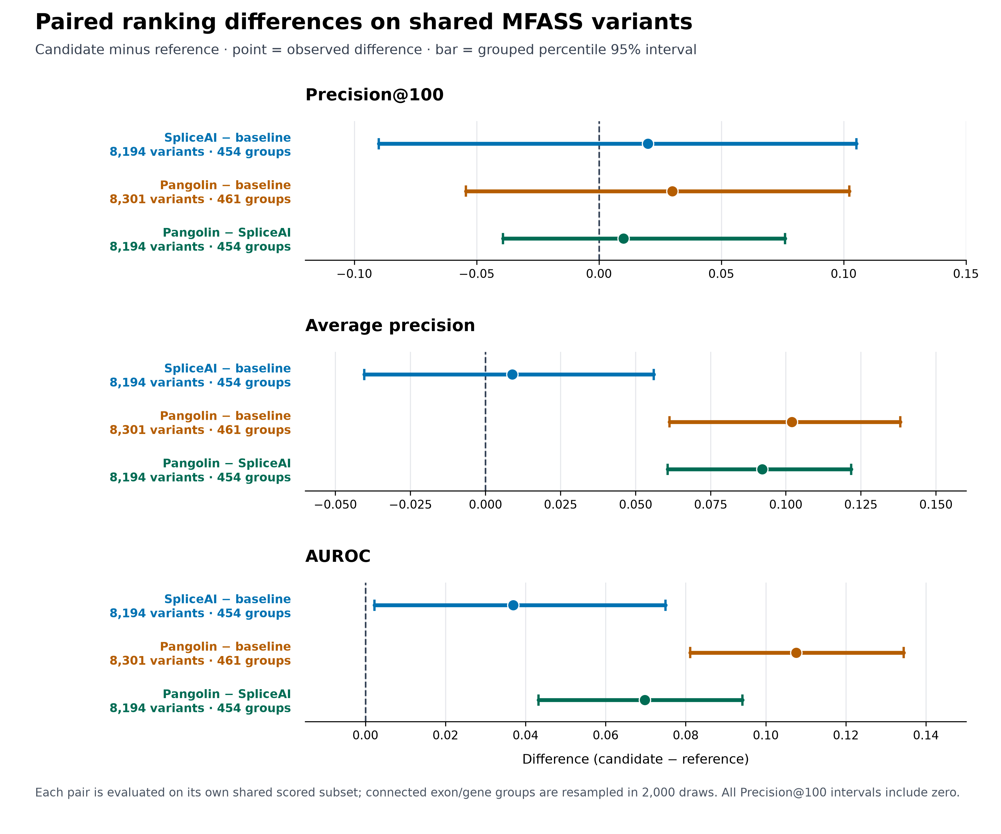
Figure 3. Dots are observed paired differences on shared scored variants; bars are grouped percentile 95% intervals from 2,000 draws. Every precision@100 comparison and SpliceAI-minus-baseline AP interval spans zero; Pangolin's AP and AUROC intervals against both other methods lie above zero, while SpliceAI's AUROC interval against the corrected baseline now crosses zero. Sources: SpliceAI versus baseline, Pangolin versus baseline and Pangolin versus SpliceAI.

Pangolin's AP and AUROC intervals against both other methods exclude zero. SpliceAI's AP interval against the corrected baseline spans −0.039 to +0.061, and its AUROC interval spans −0.004 to +0.064. Neither establishes an improvement over this baseline. Every precision@100 interval crosses zero, including Pangolin minus SpliceAI at −0.039 to +0.076. Those intervals allow differences larger than the one-positive point gap in either direction.

An interval that includes zero does not show that the methods are equivalent. Establishing equivalence would require an acceptable difference specified in advance and an analysis precise enough to rule out larger differences. This comparison did neither.

The observed counts are 61, 64 and 65, but the uncertainty is too large to establish which method performs best at 100. A future comparison should specify the follow-up capacity and the minimum useful improvement before inspecting the scores.

Results by distance from an exon boundary

To examine performance at different distances from an exon boundary, the benchmark divides the 8,194 variants that all three methods scored, including 308 positives, into four distance bands. In the band more than 30 bases from the nearest boundary, 1,914 variants contain only 31 SDVs.

Its observed AUROC is 0.756 for the corrected baseline, 0.744 for SpliceAI and 0.844 for Pangolin. This distal band was noticed after inspecting four bands, and no grouped subgroup-comparison interval was computed. The baseline also learns from distance features and MFASS labels. These descriptive results cannot establish that the relative performance of the methods changes with distance.

Table 4. Descriptive AUROC in distance bands on the three-method common subset, from the pinned subgroup result.

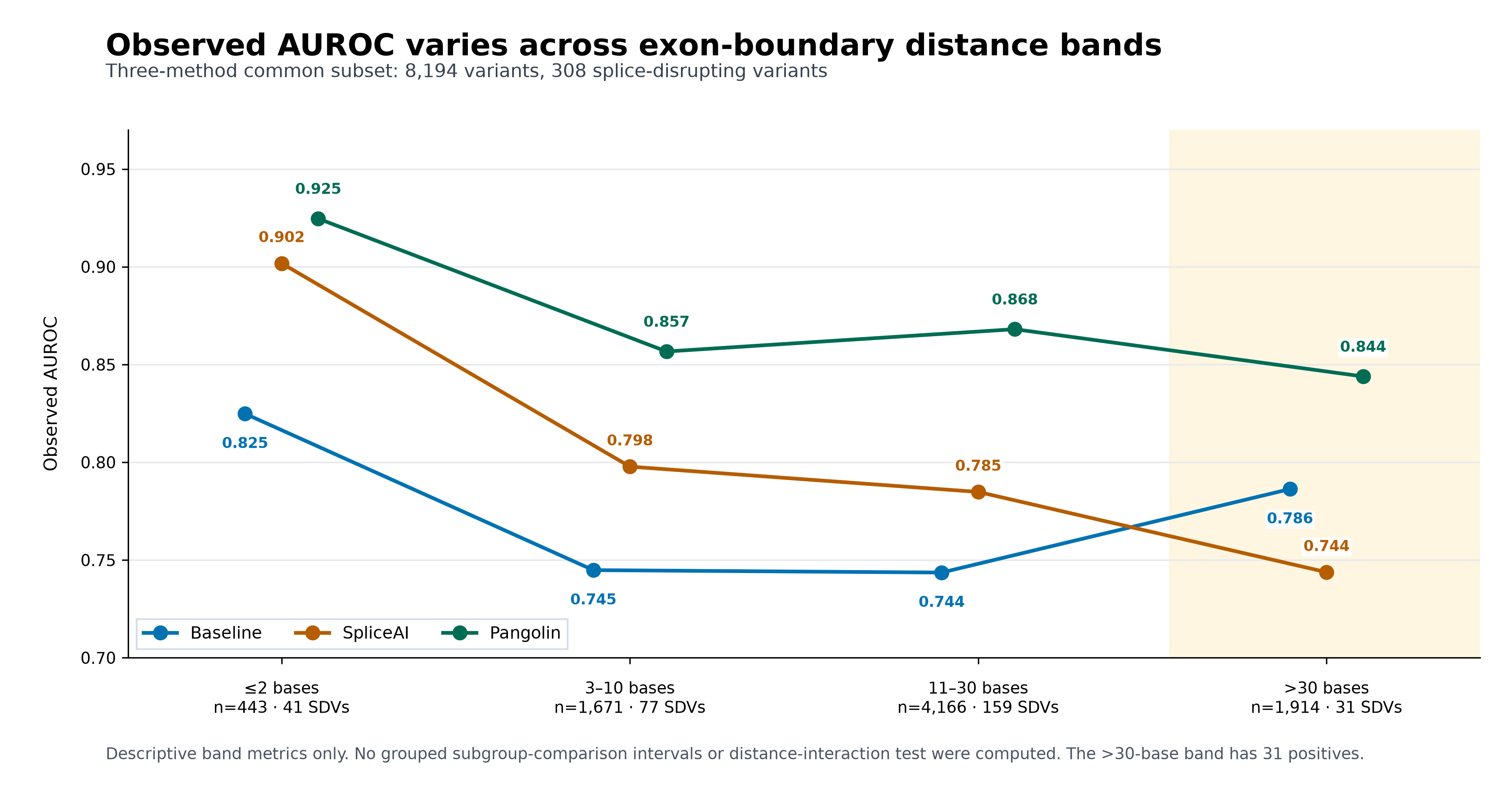
Figure 4. Descriptive AUROC on the 8,194-variant, 308-SDV three-method shared subset, stratified by nearest exon-boundary distance. This plot has no uncertainty bars or interaction test. Source: pinned subgroup result.

A future assay with more distal SDVs and matched annotations could test whether the ordering persists.

Missing scores and runtime

SpliceAI scored 8,194 of 8,324 test variants; its 130 unscored rows were logged as having no overlapping annotated gene. Pangolin scored 8,301 and skipped 23 under a catch-all reason covering no gene, reference mismatch or unsupported input. Its artifact does not disaggregate those causes. The baseline scored all 8,324.

SpliceAI's scored set includes 308 of the holdout's 315 SDVs; Pangolin's includes 314. The unscored-row artifacts matter for deployment planning alongside the score table. A workflow needs a fallback or an explicit unranked bucket for a variant the scorer declines to score.

The paired analysis compares ranking where both methods scored a variant. A method might have good AP among eligible variants and still leave important cases out of its queue. Deployment should report ranking and coverage together.

Elapsed time is useful but must be read as workflow time. On the recorded macOS arm64 machine, the corrected baseline took 1.399 seconds end to end, including cohort/split loading and validation, feature construction, fitting, prediction and result-metric computation. It excludes input downloads, cohort construction, environment installation and the post-hoc paired bootstrap. This replaces the historical baseline timing, which covered a narrower set of stages. The unchanged specialist records report SpliceAI model/reference loading plus test scoring totalling 4,463.805 seconds; Pangolin loading and test scoring totalled 13,664.821 seconds.

The baseline's recorded per-input denominator is the full 27,733-row cohort because its workflow trains and predicts; each specialist's denominator is the 8,324 test inputs. These numbers do not support a pure neural-inference speed ratio or a portable cost prediction. They do say that the reported specialist workflows required substantially more wall time on this machine, and a production choice should be timed with its actual batching, hardware and reference assets.

Reproducing the results

The public benchmark snapshot at commit bee9133b83f3aedaf2bbb9013f1875515845607e was checked on 16 September 2026. The core install, cohort validation, baseline, three paired comparisons and subgroup commands were executed in an isolated archive of that exact revision. The fresh-clone setup below is provided for readers; the verification used git archive from the local repository instead of a new clone. No specialist inference was rerun.

Both author tables were freshly downloaded from revision 9a8e4f27106be52aeb11acad27f95f5cded663a8 and their hashes verified. The functional-annotation table supplies gene and conservation information required by the split and baseline. Compare the three printed SHA-256 digests with these values before continuing:

• snv_data_clean.txt: a637ca0e307e66ff48811ec7efa22b9ce453bc7883b04f0cacb867f7283132d8
• snv_func_annot.txt: 71a857fe647c4e68acbb41ca61e959c47e1176de89b1442bd6ca1772aa60d5a1
• split-v2.tsv: 999ebcb7e63a5c5eaa8780fa468e59ac1f934260ad50102814174c396317f052

With Git, curl, uv and Python 3.11 available, the following uses the checked-in connected split and writes fresh outputs under the ignored data directory:

git clone https://github.com/timini/rewire-benchmarks.git
cd rewire-benchmarks
git checkout bee9133b83f3aedaf2bbb9013f1875515845607e
uv sync --frozen --package mfass --python 3.11
mkdir -p benchmarks/mfass/data/repro
curl -fL -o benchmarks/mfass/data/snv_data_clean.txt \
  https://raw.githubusercontent.com/KosuriLab/MFASS/9a8e4f27106be52aeb11acad27f95f5cded663a8/processed_data/snv/snv_data_clean.txt
curl -fL -o benchmarks/mfass/data/snv_func_annot.txt \
  https://raw.githubusercontent.com/KosuriLab/MFASS/9a8e4f27106be52aeb11acad27f95f5cded663a8/processed_data/snv/snv_func_annot.txt
shasum -a 256 benchmarks/mfass/data/snv_data_clean.txt \
  benchmarks/mfass/data/snv_func_annot.txt benchmarks/mfass/splits/split-v2.tsv
export OMP_NUM_THREADS=4
export OPENBLAS_NUM_THREADS=4
uv run --frozen --package mfass mfass-build --check
uv run --frozen --package mfass mfass-build --out benchmarks/mfass/data/repro/cohort.tsv
uv run --frozen --package mfass mfass-baseline \
  --cohort benchmarks/mfass/data/repro/cohort.tsv \
  --split benchmarks/mfass/splits/split-v2.tsv \
  --capacity 100 --seed 20260914 \
  --out benchmarks/mfass/data/repro/baseline-kmer-position-v2.json

The expected counts are 27,733 variants and 1,050 SDVs in the cohort, 1,590 connected groups, and 8,324 test variants with 315 SDVs in 463 groups. The corrected baseline reports precision@100 0.610, AP 0.286 and AUROC 0.778. A changed digest or count means a different input or split and should be investigated before comparing scores.

In this verification, the rebuilt cohort's SHA-256 was 389702ff4c647d7ce10a90092a6fa811ae777d15997baf39ce9aae0346247bd0. Independently regenerating the connected split reproduced the checked-in file byte for byte. The baseline's prediction TSV also matched the pinned v2 artifact byte for byte, and its point metrics matched at full precision. Elapsed time is run-specific and is not expected to reproduce exactly.

These comparisons use the freshly generated baseline predictions and the committed specialist predictions. All three paired result files matched the pinned numerical results exactly, including the 2,000-draw intervals; their input-path strings differ. The comparison commands were tested in an isolated output directory. The commands below write to a different directory; the bootstrap calculations were not repeated solely for that path change. The cohort and baseline commands were also run using the paths shown here.

uv run --frozen --package mfass mfass-compare \
  --baseline benchmarks/mfass/data/repro/baseline-kmer-position-v2.predictions.tsv \
  --candidate benchmarks/mfass/results/spliceai-1.3.1.predictions.tsv \
  --capacity 100 --draws 2000 --seed 20260914 --out benchmarks/mfass/data/repro/compare-baseline-v2-vs-spliceai.json
uv run --frozen --package mfass mfass-compare \
  --baseline benchmarks/mfass/data/repro/baseline-kmer-position-v2.predictions.tsv \
  --candidate benchmarks/mfass/results/pangolin-maskFalse.predictions.tsv \
  --capacity 100 --draws 2000 --seed 20260914 --out benchmarks/mfass/data/repro/compare-baseline-v2-vs-pangolin-maskFalse.json
uv run --frozen --package mfass mfass-compare \
  --baseline benchmarks/mfass/results/spliceai-1.3.1.predictions.tsv \
  --candidate benchmarks/mfass/results/pangolin-maskFalse.predictions.tsv \
  --capacity 100 --draws 2000 --seed 20260914 --out benchmarks/mfass/data/repro/compare-spliceai-1.3.1-vs-pangolin-maskFalse.json
uv run --frozen --package mfass mfass-subgroups --capacity 100 \
  --cohort benchmarks/mfass/data/repro/cohort.tsv \
  --methods baseline=benchmarks/mfass/data/repro/baseline-kmer-position-v2.predictions.tsv \
  spliceai=benchmarks/mfass/results/spliceai-1.3.1.predictions.tsv \
  pangolin=benchmarks/mfass/results/pangolin-maskFalse.predictions.tsv \
  --out benchmarks/mfass/data/repro/subgroups-canonical-v2.json

The subgroup calculation reproduced all counts and displayed three-decimal values. Five unrounded baseline metrics differed from the pinned subgroup artifact by at most 0.00000857; the cause was not established. The published table and figure use the pinned v2 JSON, not the rerun's slightly different unrounded values.

Source downloads and rerun outputs stay under the ignored benchmarks/mfass/data/ tree, preserving the committed split and results. The archived v1 snapshot remains available for inspecting the original baseline and comparisons. It is a historical record, not current evidence for choosing a model.

For full specialist scoring, the pinned benchmark scorer implementations require a GRCh38 primary-assembly FASTA, GENCODE v44 GTF and Pangolin database, model dependencies and checkpoints. SpliceAI uses its bundled v24-derived annotation for this reported run; the v44 database belongs to Pangolin and a future matched-annotation test.

The following full-run commands were inspected against current CLI flags but were not executed in this article pass. They assume the reference FASTA and database have been prepared using the linked GENCODE files and Pangolin database script. A rerun with the shown current Pangolin package pin would be a new run, because the installed commit for the historical result was not recorded.

uv sync --package mfass --extra spliceai --extra pangolin
uv pip install --python .venv/bin/python \
  'git+https://github.com/tkzeng/Pangolin.git@5cf94b8db938c658391b4305cd7ce33297d44ff7'
uv run --no-sync mfass-spliceai \
  --cohort benchmarks/mfass/data/repro/cohort.tsv \
  --split benchmarks/mfass/splits/split-v2.tsv \
  --ref benchmarks/mfass/data/ref/GRCh38.primary_assembly.genome.fa \
  --annotation grch38 --distance 50 --mask 0 \
  --out benchmarks/mfass/data/repro/spliceai-full.json
uv run --no-sync mfass-pangolin \
  --cohort benchmarks/mfass/data/repro/cohort.tsv \
  --split benchmarks/mfass/splits/split-v2.tsv \
  --ref benchmarks/mfass/data/ref/GRCh38.primary_assembly.genome.fa \
  --db benchmarks/mfass/data/ref/gencode.v44.annotation.db \
  --distance 50 --mask False \
  --out benchmarks/mfass/data/repro/pangolin-full.json

The existing Pangolin result lacks the installed upstream package commit. Checkpoint identity and scores would need reconciliation before treating a new full scorer run as a reproduction of the existing one. The tested commands use the archived specialist predictions. Specialist score generation was not rerun for this article.

What the corrected comparison supports

For this MFASS test set and these configurations, Pangolin has higher AP and AUROC than both the trained baseline and SpliceAI, with paired confidence intervals above zero. The specialists were not fitted to this run's 19,409 MFASS training labels. SpliceAI's AUROC interval against the corrected baseline crosses zero, as does its AP interval. The earlier v1 claim of clear AUROC separation is withdrawn.

At the original 100-place operating point, every paired precision@100 interval among these three methods crosses zero. The observed queues of 61, 64 and 65 positives are useful planning numbers, yet this holdout has not established which method reliably fills that queue best.

The next controlled specialist comparison should keep the connected holdout, match annotations, record Pangolin package and checkpoint provenance, regenerate coverage and pairwise tables on shared scored variants, and expand the distance analysis with more positive examples. This three-method run did not record a predeclared improvement margin; adding one now cannot make the existing comparison prospective.

A foundation-model follow-up

MFASS v2 also evaluated frozen DNABERT-2 117M embeddings with a fixed logistic head trained on the MFASS training arm. That protocol scored all 8,324 held-out variants, found 3 disruptions in its first 100, and reached AP 0.045 and AUROC 0.550. Its paired intervals against the corrected baseline favour the baseline on all three measures.

That is a result for one pooling, pair-representation and supervised-head configuration. It does not establish DNABERT-2's best achievable performance or a general verdict on genomic foundation models. The unresolved top-100 comparison above refers specifically to the original baseline, SpliceAI and Pangolin. The linked v2 report gives the separate protocol, uncertainty and pretraining-overlap limitations.

Sources and artifacts

• Chong et al., MFASS functional assay and author processed-data repository.
• Jaganathan et al., SpliceAI and official software documentation.
• Zeng and Li, Pangolin and official software documentation.
• Rentzsch et al., CADD-Splice and prior MFASS evaluation, GENCODE human release 44 and scikit-learn average precision definition.
• Corrected MFASS v2 benchmark code, split and result snapshot, commit bee9133b83f3aedaf2bbb9013f1875515845607e.