Why 1000-Layer Networks Finally Work for Reinforcement Learning

Most RL practitioners stop at 4 to 8 layers. The reasoning seems sensible: RL training is unstable enough without adding the gradient pathologies of extreme depth. Value networks stay shallow, feature extractors stay modest. But what if this assumption has been holding us back?

Recent research from Wang et al. demonstrates that scaling networks to 1024 layers achieves 2x to 50x improvements on self-supervised RL algorithms (Wang et al., 2025). The gains appear specifically in goal-conditioned settings, where agents learn to reach arbitrary target states without explicit reward engineering.

Prerequisites: This post assumes familiarity with neural network basics and reinforcement learning fundamentals. If you have trained a DQN or policy gradient agent before, you have sufficient background.

This post explains why goal-conditioned RL creates unique conditions where extreme depth pays off, walks through the architectural requirements for training 1000-layer networks, and identifies when this approach makes sense for your problems.

What Makes Goal-Conditioned RL Different

Traditional RL trains agents to maximize a fixed reward signal. Change the reward, and you retrain from scratch. Goal-conditioned RL takes a different approach: the agent learns to reach arbitrary goal states specified at test time. The policy becomes a function of both current state and desired goal.

This matters for practical applications. Consider a robot arm that needs to reach different target positions. With traditional RL, you would need separate policies for each target. With goal-conditioned RL, you train once and specify goals at deployment.

Goal-Conditioned Supervised Learning (GCSL) "provides a new learning framework by iteratively relabeling and imitating self-generated experiences" (Yang et al., 2022). This self-supervised approach eliminates reward engineering entirely.

The challenge is that goal-conditioned policies must generalize across the entire goal space. The agent needs representations capturing meaningful distances between states, not just local value estimates. This is where depth becomes crucial.

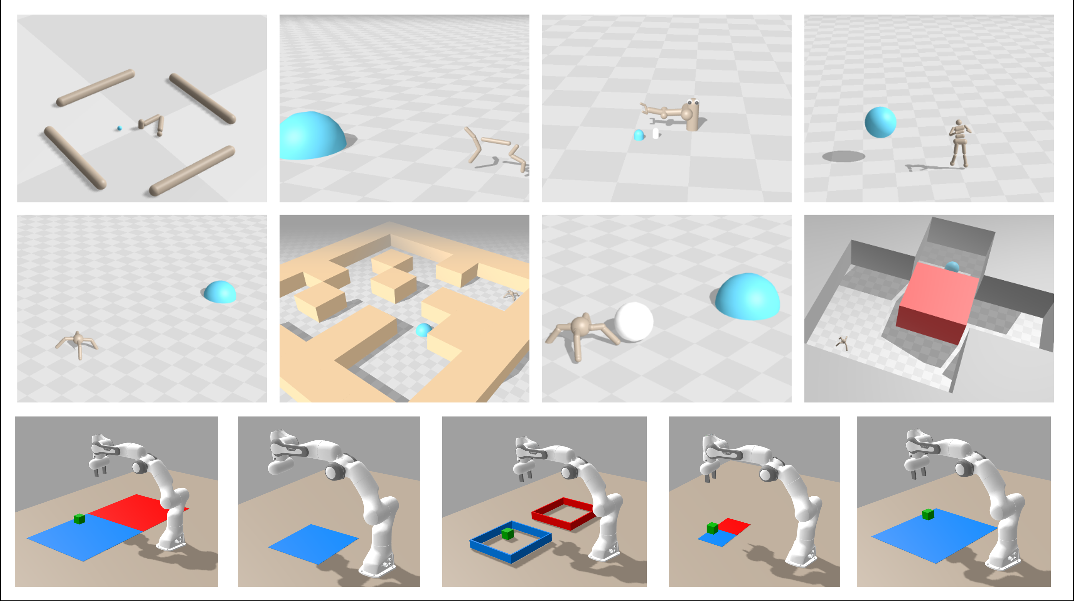Figure 1: Benchmark environments for goal-conditioned RL spanning navigation, locomotion, and manipulation. Source: 1000-Layer Networks for Self-Supervised RL, Wang et al.

These environments require agents to learn goal-reaching policies that generalize to positions never seen during training.

Why Contrastive Learning Enables Depth Scaling

Here is where depth scaling becomes relevant. Contrastive learning provides a natural objective for goal-conditioned RL that benefits from hierarchical feature extraction.

The core insight comes from Eysenbach and Levine (2022): "contrastive representation learning can be formulated as goal-conditioned RL, where learned representations correspond exactly to goal-conditioned value functions."

In practice, the contrastive objective learns representations where states close in achievability cluster together, while distant states spread apart. This is precisely what a goal-conditioned value function should capture: how "far" the current state is from the goal in terms of actions needed to reach it.

CURL demonstrated this connection empirically, achieving "1.9x performance gain at 100K environment steps on DMControl" through contrastive learning combined with standard off-policy RL (Laskin et al., 2020).

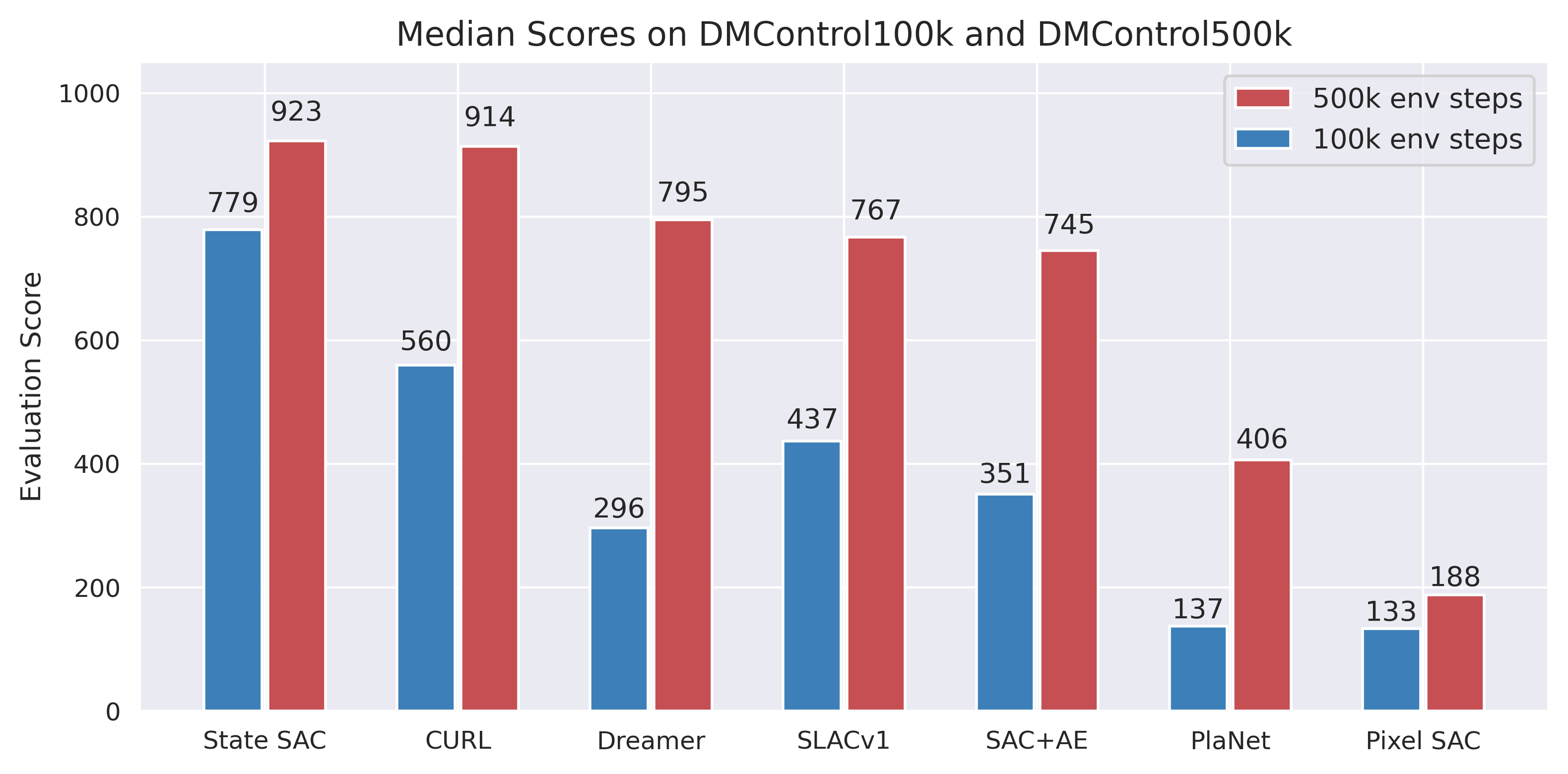Figure 2: CURL benchmark results showing contrastive learning closing the gap with state-based methods. Source: CURL: Contrastive Unsupervised Representations for RL, Laskin et al.

The question becomes: if contrastive objectives benefit from representation learning, and deep networks excel at hierarchical feature extraction, why stop at 4 or 8 layers?

Why Shallow Networks Fail at Complex Goal-Reaching

Standard RL networks use 2 to 4 fully connected layers. This works for simple control tasks where the optimal policy depends on local state information. Goal-conditioned tasks demand something different.

Consider maze navigation. A shallow network can learn local gradients: move right when the goal is to the right. But obstacles block direct paths. The optimal action might be moving away from the goal temporarily to navigate around a wall.

This requires understanding global structure, not just local gradients. The network must learn that certain state-action sequences eventually lead to the goal even when immediate progress appears negative.

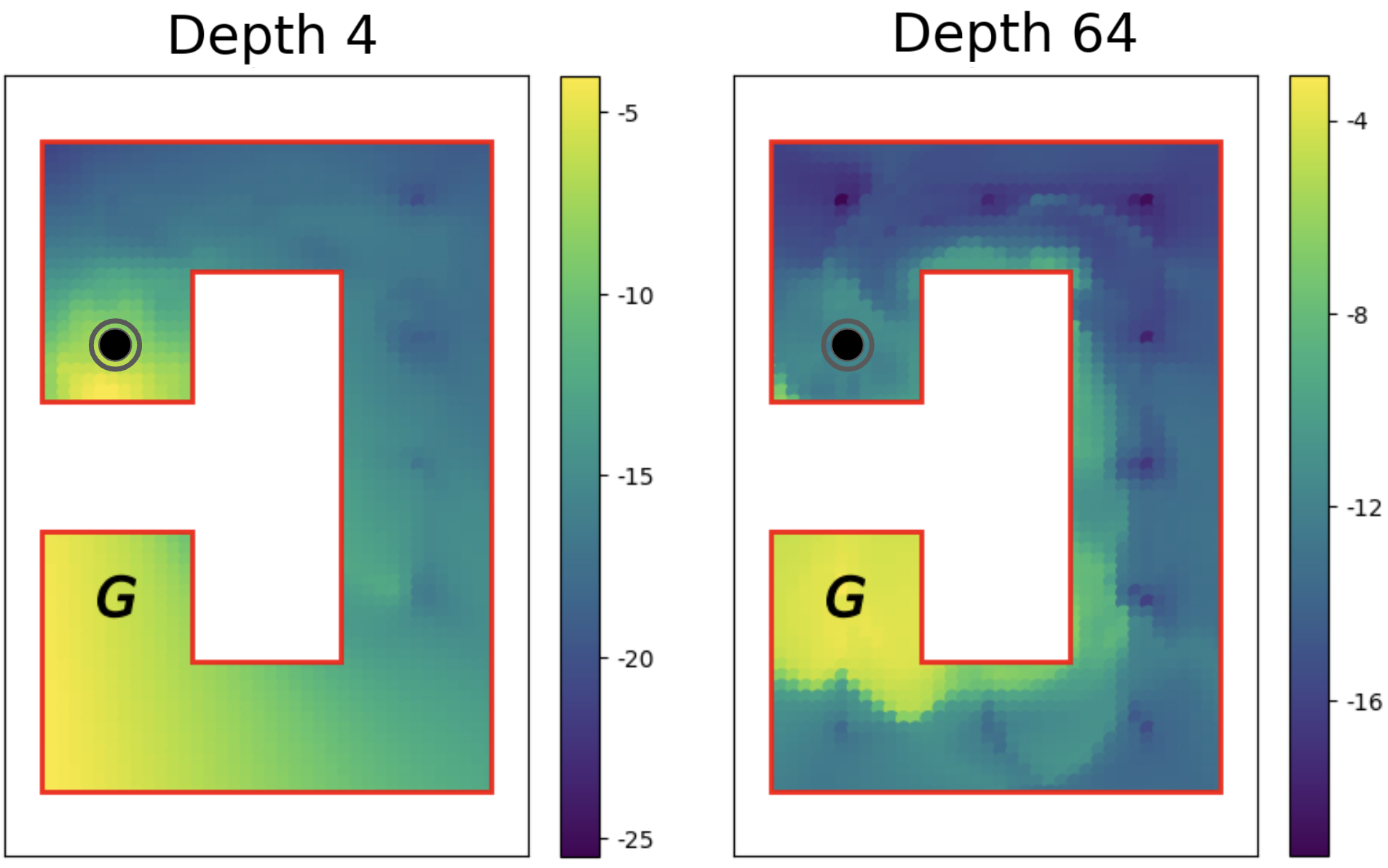Figure 3: Value function comparison showing how deeper networks capture obstacle structure that shallow networks miss. Source: 1000-Layer Networks for Self-Supervised RL, Wang et al.

The heatmaps reveal the difference. At depth 4, the value function shows rough, discontinuous estimates around obstacles. At depth 64, the network learns smooth gradients that correctly capture path structure. The deeper network understands that states on opposite sides of a wall have very different goal-reaching difficulties, even when spatially close.

From supervised learning, "the Universal Approximation Theorem underpins the expressivity of neural networks: a two-layer network can already approximate any measurable function arbitrarily well" (Policy Gradients Guide). But approximation quality differs from learning efficiency. Deep networks learn smoother functions that generalize better and train more stably.

The Architecture That Makes 1000 Layers Trainable

Extreme depth requires architectural support for gradient flow. The key innovation is residual connections combined with proper normalization.

"ResNets represented a major milestone in deep learning by successfully addressing the vanishing gradient problem through skip connections" (Timushev et al., 2024). But residual connections alone are insufficient at extreme depths. "Skip connections in ResNets can lead to gradient overlap, where gradients from both the learned transformation and the skip connection combine, potentially resulting in overestimated gradients."

The solution combines multiple techniques. Layer normalization ensures consistent activation scales across depths. "Layer normalization performs exactly the same computation at training and test times" (Ba et al., 2016), avoiding batch-size dependencies that plague batch normalization in RL settings.

"""
Deep Residual Block with Layer Normalization for RL Networks

Uses pre-layer normalization pattern which enables stable training
at 1000+ layer depths. Key: LayerNorm BEFORE activation, not after.
"""

import torch
import torch.nn as nn


class DeepResidualBlock(nn.Module):
    """
    Residual block with pre-layer normalization for deep RL networks.
    Pattern: x + f(LayerNorm(x)) provides better gradient flow than
    post-normalization: LayerNorm(x + f(x))
    """

    def __init__(self, hidden_dim: int, dropout: float = 0.0):
        super().__init__()
        self.norm = nn.LayerNorm(hidden_dim)
        self.fc1 = nn.Linear(hidden_dim, hidden_dim)
        self.fc2 = nn.Linear(hidden_dim, hidden_dim)
        self.activation = nn.ReLU()
        self.dropout = nn.Dropout(dropout) if dropout > 0 else nn.Identity()

        # Initialize for stable deep training
        nn.init.xavier_uniform_(self.fc1.weight)
        nn.init.xavier_uniform_(self.fc2.weight)
        nn.init.zeros_(self.fc2.bias)  # Zero init for residual output

    def forward(self, x: torch.Tensor) -> torch.Tensor:
        residual = x
        x = self.norm(x)           # Pre-layer normalization
        x = self.activation(self.fc1(x))
        x = self.dropout(x)
        x = self.fc2(x)
        return residual + x        # Skip connection


# Usage: Stack 64 blocks for a 128-layer network
network = nn.Sequential(
    nn.Linear(64, 256),  # Input projection
    *[DeepResidualBlock(256) for _ in range(64)],
    nn.LayerNorm(256),
    nn.Linear(256, 4)    # Output (e.g., action dim)
)

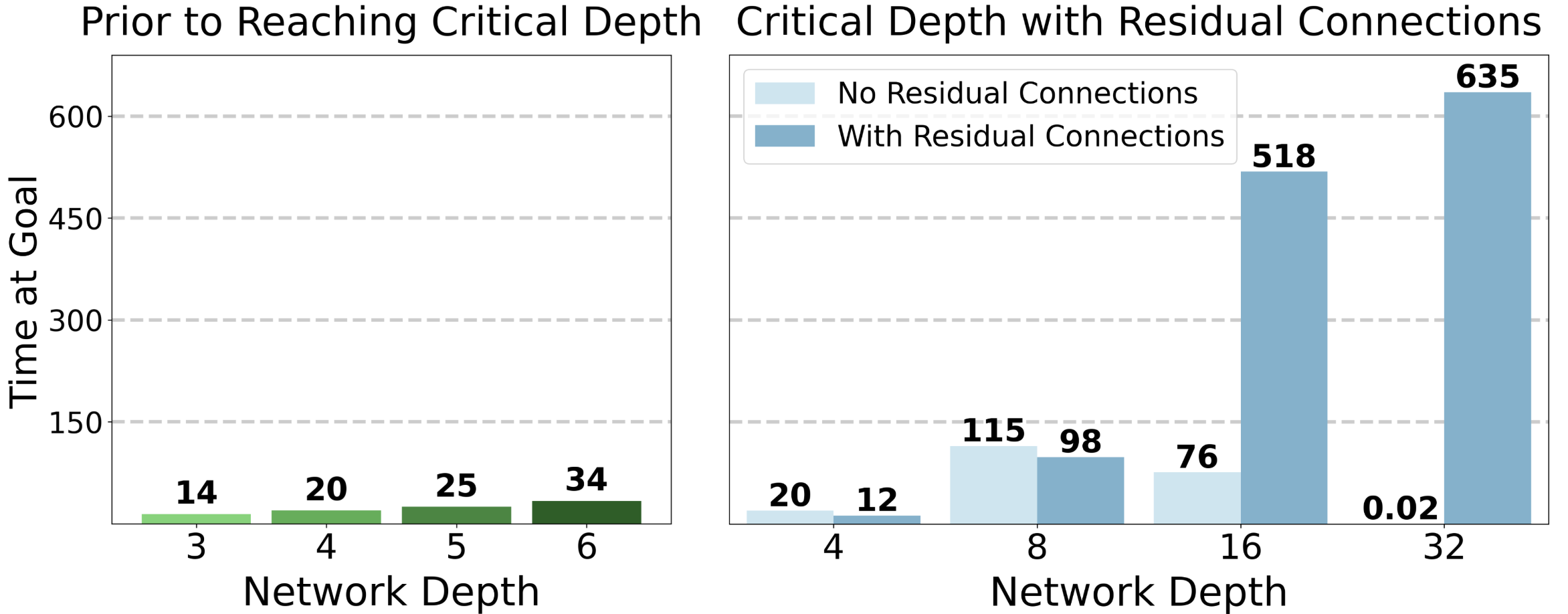Figure 4: Critical depth analysis showing residual connections enable deep RL networks. Source: 1000-Layer Networks for Self-Supervised RL, Wang et al.

The chart shows the dramatic impact. Without residual connections, performance collapses completely at 32 layers. With residual connections, performance not only remains stable but continues improving as depth increases. The difference at depth 32 is not incremental; it is the difference between a functioning agent and complete failure.

Gradient normalization provides additional stability. "ZNorm adjusts the gradient scale, standardizing gradients across layers and reducing the negative impact of overlapping gradients" (Timushev et al., 2024). This keeps gradient magnitudes consistent through all 1000 layers.

Generalization Benefits Beyond Training Performance

The performance improvements are not just about fitting the training distribution better. Deeper networks show improved generalization to novel goals.

This matters because goal-conditioned RL must handle goals at test time that differ from training. A policy that memorizes training goals provides no value; the whole point is generalization.

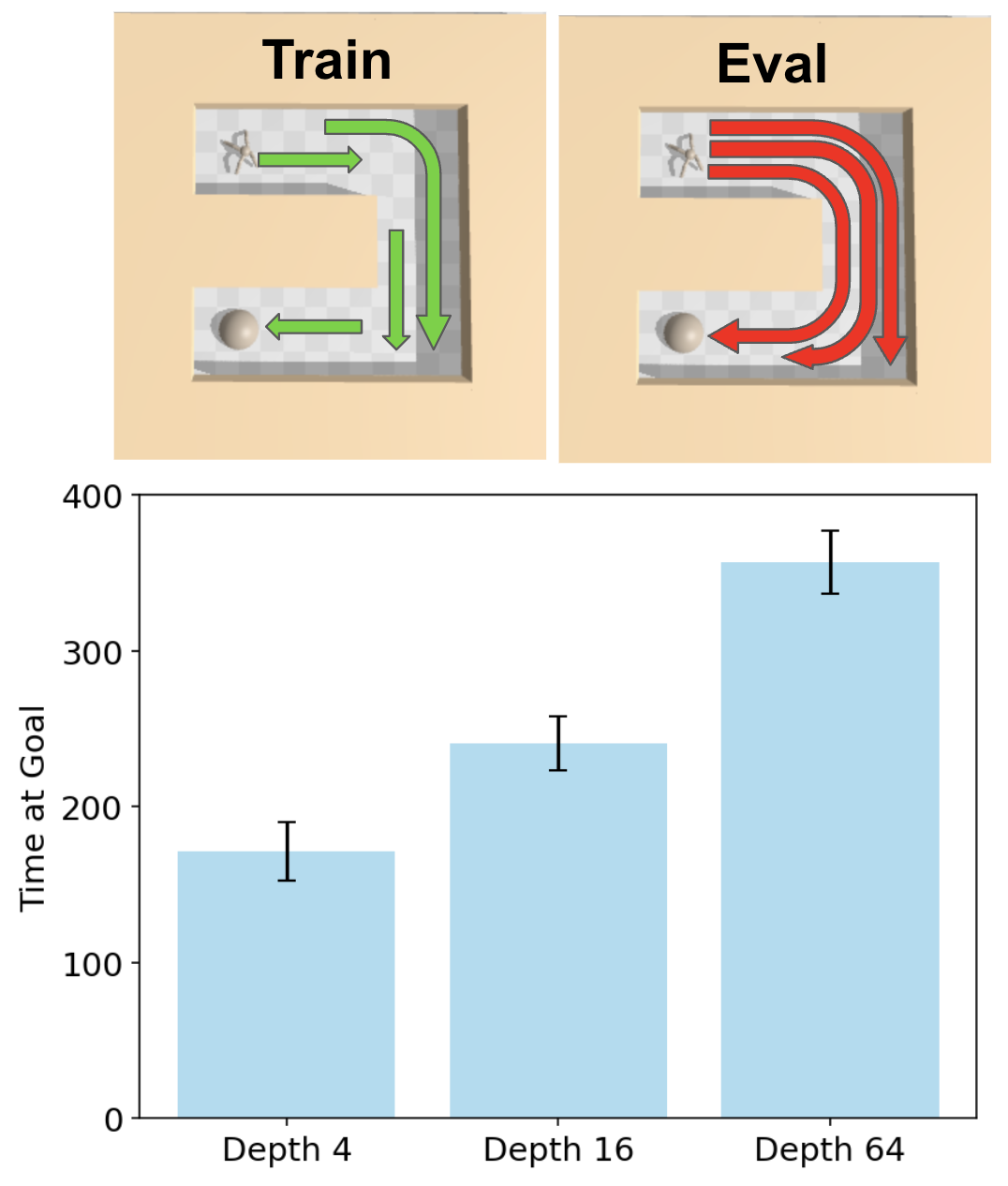Figure 5: Train vs evaluation generalization showing depth improves novel goal performance. Source: 1000-Layer Networks for Self-Supervised RL, Wang et al.

The experiment evaluates on goal positions explicitly excluded from training (red paths) while training only on the opposite direction (green paths). Deeper networks show nearly 2x improvement on these held-out goals, demonstrating that depth improves generalization rather than memorization.

Why does this happen? The contrastive learning hypothesis suggests deep networks learn more abstract, compositional representations of state relationships. These representations capture general principles of reachability that transfer across the goal space.

Practical Implementation Considerations

Building and training 1000-layer RL networks requires attention to several practical details.

Memory Management

A 1024-layer network consumes significant GPU memory. Gradient checkpointing trades computation for memory by recomputing intermediate activations during the backward pass instead of storing them. The authors report training on standard research hardware, suggesting feasibility with careful implementation.

Training Stability

Proper initialization is essential. The DeepNet work on Transformers demonstrates that "a theoretically-justified normalization function applied to residual connections enables stable training of extremely deep networks" (Wang et al., 2022). Similar principles apply to feedforward networks in RL.

"""
Gradient Monitoring for Deep RL Networks

Detects vanishing/exploding gradients and provides early warnings
during training of 1000-layer networks.
"""

import torch
import torch.nn as nn
from typing import Dict, List, Tuple
from collections import defaultdict


class GradientMonitor:
    """Monitor gradient statistics across network layers."""

    def __init__(
        self,
        model: nn.Module,
        clip_threshold: float = 1.0,
        vanishing_threshold: float = 1e-7,
        exploding_threshold: float = 1e3
    ):
        self.model = model
        self.clip_threshold = clip_threshold
        self.vanishing_threshold = vanishing_threshold
        self.exploding_threshold = exploding_threshold

    def check_gradient_health(self) -> Tuple[bool, List[str]]:
        """Check for gradient pathologies across all layers."""
        warnings = []
        is_healthy = True

        for name, param in self.model.named_parameters():
            if param.grad is None:
                continue

            grad_norm = param.grad.norm().item()

            if grad_norm < self.vanishing_threshold:
                warnings.append(f"VANISHING: {name} (norm={grad_norm:.2e})")
                is_healthy = False

            if grad_norm > self.exploding_threshold:
                warnings.append(f"EXPLODING: {name} (norm={grad_norm:.2e})")
                is_healthy = False

            if torch.isnan(param.grad).any():
                warnings.append(f"NaN DETECTED: {name}")
                is_healthy = False

        return is_healthy, warnings

    def clip_and_monitor(self) -> Dict[str, float]:
        """Clip gradients and return monitoring statistics."""
        total_norm = torch.nn.utils.clip_grad_norm_(
            self.model.parameters(), self.clip_threshold
        )
        return {
            "total_norm": total_norm.item() if torch.is_tensor(total_norm) else total_norm,
            "clipped": total_norm > self.clip_threshold,
            "clip_threshold": self.clip_threshold
        }


# Usage in training loop
def train_with_monitoring(model, optimizer, loss, monitor, step):
    optimizer.zero_grad()
    loss.backward()

    is_healthy, warnings = monitor.check_gradient_health()
    clip_stats = monitor.clip_and_monitor()

    if not is_healthy:
        print(f"Step {step} warnings: {warnings[:3]}")
    if clip_stats["clipped"]:
        print(f"Step {step}: Gradients clipped (norm {clip_stats['total_norm']:.2f})")

    optimizer.step()
    return {"loss": loss.item(), "grad_norm": clip_stats["total_norm"]}

Hyperparameter Sensitivity

Deeper networks are more sensitive to learning rates. Start with smaller learning rates (0.1x to 0.01x of shallow network defaults) and use learning rate warmup over the first 10% of training.

Computational Cost

The cost is real but manageable. "PWM trains policies for 10k gradient steps, which take 9.3 minutes on an Nvidia RTX 6000 GPU" (PWM paper, 2024). Deeper networks add proportional overhead without changing the fundamental training loop.

When Extreme Depth Makes Sense

Not every RL problem benefits from 1000 layers. The gains appear specifically in settings with these characteristics:

Self-supervised or contrastive objectives: Contrastive learning provides the training signal that deep networks exploit. Standard reward-based RL may not see the same benefits.

Goal-conditioned policies: The need to generalize across goal space creates representational demands that shallow networks struggle with.

Complex environment structure: Mazes, obstacles, and multi-step dependencies create conditions where hierarchical representations provide value.

Sufficient training data: Deep networks require more samples to train effectively. The self-supervised setting generates this data through exploration.

For standard Atari games or simple continuous control, shallow networks remain appropriate. The depth scaling results are specific to the goal-conditioned contrastive learning setting.

Open Research Questions

Several directions remain unexplored.

What is the optimal depth for a given task? The current work shows performance improves with depth but does not identify saturation points. Do different tasks have different optimal depths? Can we predict optimal depth from task properties?

How does depth interact with other architectural choices? Research on network sparsity suggests it "can unlock deeper scaling potential in RL by reducing pathologies associated with extremely deep dense networks." What combinations of depth, width, sparsity, and attention mechanisms produce the best results?

Can depth replace other complexity? If depth enables better representations, can we simplify other parts of the RL pipeline? Simpler reward functions? Less environment engineering?

Going Deeper

The 1000-layer RL research opens several directions worth exploring.

Original paper and code: The full paper (Wang et al., 2025) is available at arXiv:2503.14858 with implementation details and additional experiments.

Background on contrastive RL: Eysenbach and Levine's work establishing the connection between contrastive learning and goal-conditioned RL provides theoretical foundations. Read Contrastive Learning as Goal-Conditioned RL for the mathematical framework.

JaxGCRL for fast experiments: Myers et al. provide a high-performance implementation achieving "22x speedup in training on single GPU compared to prior implementations" (Myers et al., 2024). This enables rapid prototyping of deep goal-conditioned agents.

Experiment to try: Take an existing goal-conditioned RL implementation and systematically increase network depth while adding residual connections and layer normalization. Track both training stability (gradient norms, loss curves) and evaluation performance on held-out goals. The transition from shallow to deep should reveal the inflection point where additional depth provides consistent gains.

---

References

Ba, J. L., Kiros, R., & Hinton, G. E. (2016). Layer Normalization. arXiv preprint arXiv:1607.06450.

Eysenbach, B., & Levine, S. (2022). Contrastive Learning as Goal-Conditioned Reinforcement Learning. Advances in Neural Information Processing Systems (NeurIPS).

Laskin, A., Lee, K., Stooke, A., Pinto, L., & Abbeel, P. (2020). CURL: Contrastive Unsupervised Representations for Reinforcement Learning. International Conference on Learning Representations (ICLR).

Myers, V., Raji, I., & Eysenbach, B. (2024). Accelerating Goal-Conditioned RL Algorithms and Research. arXiv preprint arXiv:2408.11052.

Tassa, Y., Doron, Y., Muldal, A., Erez, T., Li, Y., de Las Casas, D., ... & Riedmiller, M. (2018). DeepMind Control Suite. arXiv preprint arXiv:1801.00690.

Timushev, A., Spillman, O., Jiang, T., & Sastry, S. (2024). Mitigating Gradient Overlap in Deep Residual Networks. arXiv preprint arXiv:2410.21564.

Wang, H., et al. (2022). DeepNet: Scaling Transformers to 1,000 Layers. IEEE Transactions on Pattern Analysis and Machine Intelligence.

Wang, K., Javali, I., Bortkiewicz, M., Trzcinski, T., & Eysenbach, B. (2025). 1000 Layer Networks for Self-Supervised RL: Scaling Depth Can Enable New Goal-Reaching Capabilities. arXiv preprint arXiv:2503.14858.

Yang, R., et al. (2022). Rethinking Goal-Conditioned Supervised Learning and Its Connection to Offline RL. arXiv preprint arXiv:2202.04478.