Using Embedding Models to Predict Sentence Complexity

Can a computer tell if a sentence is easy or hard to read? For decades, we've relied on simple formulas that count syllables and measure sentence length. But consider these two sentences: "The cat sat on the mat" scores easier than "Quantum entanglement enables instant correlation." The first formula gives us a grade-level score. The second describes a profoundly complex physics concept. Yet by traditional metrics, they might score similarly.

This tension between surface-level proxies and actual comprehension difficulty has driven researchers to explore a radically different approach: representing sentences as high-dimensional vectors and using machine learning to predict their complexity. But does geometry capture grammar? Can the distance between two points in a 384-dimensional space tell us if a sentence will confuse a reader?

What We Mean When We Say "Complex"

Before we can measure complexity, we need to define it precisely. The term turns out to be more slippery than it first appears.

Linguists distinguish between two fundamentally different notions of complexity. Relative complexity is subjective - it measures how difficult you find a sentence based on your background, vocabulary, and cognitive state. Absolute complexity, by contrast, is an objective property of the linguistic structure itself, independent of any reader.

Think of it this way: a legal contract written in simple English might be absolutely simple (short words, basic grammar) but relatively complex for a non-lawyer because of unfamiliar concepts. Conversely, a sentence like "DNA polymerase synthesizes nucleotide chains" is absolutely complex (technical terminology, abstract process) but relatively simple for a molecular biologist.

This research focuses on absolute complexity because it's measurable and consistent across contexts. But even absolute complexity isn't monolithic. A sentence can be complex in at least four distinct ways:

Syntactic complexity captures structural intricacy. Consider the difference between "The dog barks" and "The dog that chased the cat that ate the mouse barks." Both describe a barking dog, but the second embeds multiple subordinate clauses in a recursive structure that taxes your working memory. When linguists analyze syntactic complexity, they build parse trees - hierarchical diagrams showing how words group into phrases and clauses. Deeper trees mean more complex syntax.

Semantic complexity measures meaning density. A sentence discussing abstract philosophical concepts like "epistemological frameworks constrain interpretative methodologies" packs more semantic content than "I went to the store." Even if both sentences have similar lengths and structures, the first demands more cognitive effort to process.

Lexical complexity zooms in on vocabulary. It's not just about using "big words" - it's about diversity and sophistication. The ratio of unique words to total words (called Type-Token Ratio) gives a crude measure, but better metrics like MTLD (Measure of Textual Lexical Diversity) account for text length by tracking how quickly vocabulary variety drops off as you read.

Content complexity takes an information-theoretic view, counting and analyzing the distribution of entities like people, places, and organizations. A text that mentions 20 different companies across varied industries has higher content complexity than one repeatedly referencing the same three entities.

The progression from surface metrics to structural analysis isn't just about getting better numbers. It represents a shift in how we computationally define complexity itself.

The Old Guard: Syllables and Sentences

For most of the 20th century, measuring text difficulty meant counting surface features. The Flesch-Kincaid formulas became the gold standard, appearing in everything from newspaper style guides to Microsoft Word.

The Flesch Reading Ease formula spits out a 100-point score. Higher numbers mean easier text. A score of 90-100 is readable by an 11-year-old. Below 30, you need a university education. The math is straightforward:

FRE = 206.835 - 1.015 × (words/sentences) - 84.6 × (syllables/words)

The Flesch-Kincaid Grade Level variant maps this to U.S. school grades:

FKGL = 0.39 × (words/sentences) + 11.8 × (syllables/words) - 15.59

Let's see these formulas in action on real sentences:

import textstat

sentences = {
    "Simple": "The cat sat on the mat.",
    "Moderate": "Machine learning algorithms can identify patterns in large datasets.",
    "Complex": "The implementation of bidirectional encoder representations from transformers necessitates substantial computational resources."
}

for label, text in sentences.items():
    fk_grade = textstat.flesch_kincaid_grade(text)
    fre_score = textstat.flesch_reading_ease(text)
    print(f"{label}: FK Grade {fk_grade:.1f}, FRE {fre_score:.1f}")

Output:

Simple: FK Grade -1.4, FRE 116.1
Moderate: FK Grade 11.5, FRE 28.5
Complex: FK Grade 27.5, FRE -73.8

That complex sentence scores at grade 27.5 - implying you'd need to be 9 years into a PhD to understand it. The formula breaks down because it only knows two things: average sentence length and average syllables per word.

The problems run deeper than just funny numbers. These formulas ignore critical factors that affect comprehension: sentence structure, word familiarity versus word length, logical coherence, and domain-specific terminology. You can game them trivially - split one long sentence into three short ones and watch your score improve, even if meaning becomes fragmented. Use simple words in complex grammar and you'll score as "easy" despite being incomprehensible.

A UX Matters analysis lists seven fundamental flaws with these formulas, but the core issue is this: they're proxies mistaken for reality. Longer sentences correlate with difficulty, but they don't cause it. The underlying structure causes both.

From Counting to Structure: Parse Trees and Probes

If surface features fail, can we directly measure structural complexity? Yes, but it requires building parse trees - formal diagrams of a sentence's grammatical structure.

A parse tree for "The dog chased the cat" shows a simple, shallow hierarchy. But "The dog that the cat that the mouse bit chased barked" creates a deeply nested structure that mirrors the recursion inherent in human language. Computational linguists extract metrics from these trees: tree depth (how many layers of embedding), branching factor (how many children each node has), and Yngve scores (modeling working memory load during incremental processing).

The L2 Syntactic Complexity Analyzer automates this, computing 14 different syntactic metrics including clause length, subordination depth, and phrasal complexity. This is powerful, but it comes at a cost. Parsing is computationally expensive and error-prone, especially on messy real-world text. More fundamentally, these metrics still only capture syntax. What about meaning?

This is where neural networks enter the picture. Not as predictors, but as representation learners.

The Embedding Revolution: From Words to Vectors

Modern NLP shifted the paradigm from handcrafted features to learned representations. The core idea is deceptively simple: represent words and sentences as points in a high-dimensional vector space where semantic relationships correspond to geometric relationships.

Word embeddings like Word2Vec started this revolution in the 2010s. By training a neural network to predict words from their contexts, researchers discovered that the resulting vectors exhibited striking algebraic properties. The famous example: vector(king) - vector(man) + vector(woman) ≈ vector(queen). Semantic relationships became vector arithmetic.

But Word2Vec has a fatal flaw: it's context-independent. The word "bank" gets one vector whether you're talking about a financial institution or a river's edge. And averaging word vectors to represent a sentence throws away all information about word order. "The dog chased the cat" and "The cat chased the dog" would have nearly identical embeddings despite opposite meanings.

This necessitated models that could process entire sentences while maintaining context. Enter BERT.

BERT: Bidirectional Context at Scale

BERT (Bidirectional Encoder Representations from Transformers) changed everything in 2018. Unlike previous models that read text left-to-right, BERT's self-attention mechanism lets every word "see" every other word simultaneously. This bidirectional context creates rich, nuanced representations.

BERT learns through two clever pre-training tasks on massive text corpora:

1. Masked Language Modeling: Randomly hide 15% of words and train the model to predict them from surrounding context. This forces it to learn deep relationships between words.

2. Next Sentence Prediction: Given two sentences A and B, predict if B actually follows A in the original text. This teaches sentence-level relationships.

But here's the catch: when researchers tried using BERT's outputs directly as sentence embeddings, the results were surprisingly poor. Two obvious approaches failed:

• Using the hidden state of the special [CLS] token (designed to aggregate sentence meaning)
• Averaging all token embeddings (mean pooling)

Both were often beaten by simply averaging static GloVe word vectors - a technique from 2014. Why? Because BERT was trained to predict masked tokens and sentence adjacency, not to create a space where cosine similarity measures semantic similarity. The objectives don't align with the downstream use case.

SBERT: Fine-Tuning for Semantic Similarity

Sentence-BERT (SBERT) solved this problem through architectural innovation and targeted fine-tuning. Instead of processing sentence pairs together (expensive), SBERT uses a Siamese network: two identical BERT encoders with shared weights that process sentences independently and output fixed-size embeddings.

The magic happens during fine-tuning. SBERT trains on sentence-pair datasets like the Stanford Natural Language Inference corpus, which labels pairs as entailment, contradiction, or neutral. Using a contrastive loss function, the model learns to minimize distance between similar sentences (entailments) and maximize distance between dissimilar ones (contradictions).

This explicitly restructures the embedding space so that cosine similarity becomes meaningful. Let's see this in practice:

from sentence_transformers import SentenceTransformer
from sklearn.metrics.pairwise import cosine_similarity

model = SentenceTransformer('all-MiniLM-L6-v2')

sentences = [
    "The cat sat on the mat.",
    "Machine learning algorithms can identify patterns in large datasets.",
    "The implementation of bidirectional encoder representations necessitates substantial computational resources."
]

embeddings = model.encode(sentences)
similarities = cosine_similarity(embeddings)

print("Cosine Similarity Matrix:")
print(f"Simple ↔ Moderate: {similarities[0][1]:.4f}")
print(f"Simple ↔ Complex:  {similarities[0][2]:.4f}")
print(f"Moderate ↔ Complex: {similarities[1][2]:.4f}")

Output:

Simple ↔ Moderate: -0.0628
Simple ↔ Complex:  -0.0238
Moderate ↔ Complex: 0.0700

The two technical sentences (Moderate and Complex) show the highest similarity (0.07), while the simple sentence is less similar to both. The embeddings capture semantic clustering even without explicit complexity labels.

Notice that all embeddings have L2 norm = 1.0. This normalization is standard practice - without it, sentence length can dominate similarity calculations, creating spurious correlations.

Can Geometry Predict Grammar?

We have 384-dimensional vectors representing sentences. Can we extract complexity from their geometric properties?

The intuition is compelling: maybe complex sentences, with richer semantic content and more intricate structure, occupy different regions of embedding space than simple sentences. Let's visualize this directly by reducing embeddings to 2D using PCA (Principal Component Analysis):

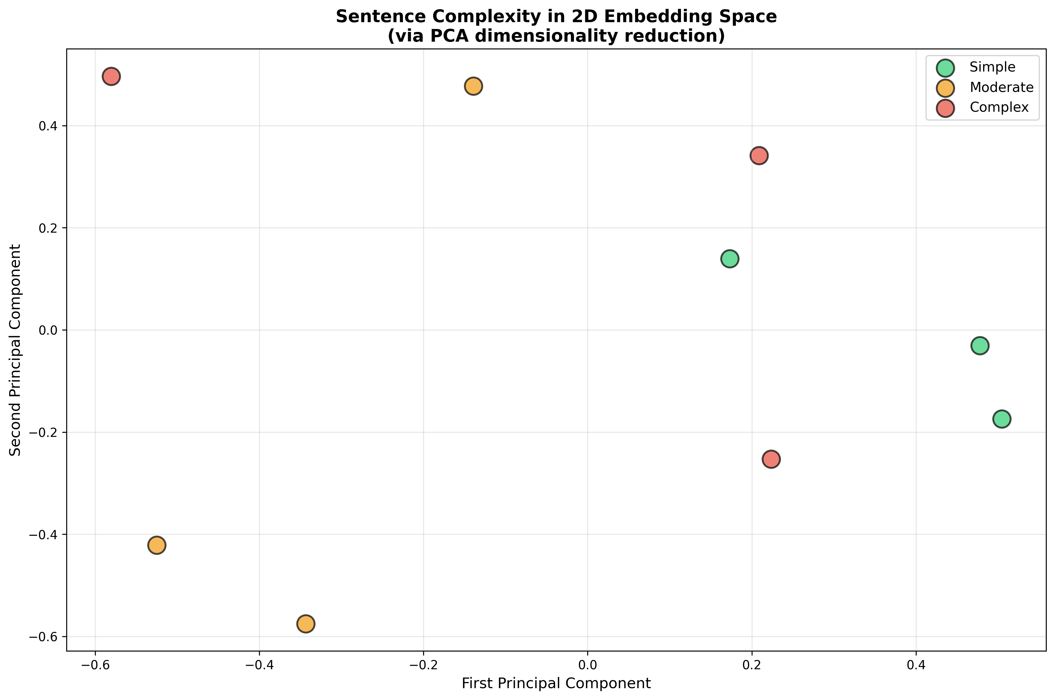
Figure 1: Nine sentences projected from 384D to 2D space via PCA. Simple sentences (green) cluster separately from moderate (orange) and complex (red) technical sentences. Only 34% of variance is captured in 2D, but visual separation suggests embeddings encode complexity signals.

from sentence_transformers import SentenceTransformer
from sklearn.decomposition import PCA
import matplotlib.pyplot as plt

sentences = [
    "I eat food.", "The dog barks.", "She reads books.",
    "Scientists study climate change effects.",
    "The algorithm processes data efficiently.",
    "Renewable energy reduces carbon emissions.",
    "The implementation of bidirectional transformers necessitates substantial computational resources.",
    "Quantum entanglement facilitates instantaneous correlation between spatially separated particles.",
    "Epistemological frameworks constrain interpretative methodologies in hermeneutic analysis."
]

complexity_labels = ["Simple"]*3 + ["Moderate"]*3 + ["Complex"]*3

model = SentenceTransformer('all-MiniLM-L6-v2')
embeddings = model.encode(sentences)

pca = PCA(n_components=2)
embeddings_2d = pca.fit_transform(embeddings)

plt.figure(figsize=(12, 8))
colors = {"Simple": "#2ecc71", "Moderate": "#f39c12", "Complex": "#e74c3c"}
for complexity in ["Simple", "Moderate", "Complex"]:
    mask = [label == complexity for label in complexity_labels]
    plt.scatter(embeddings_2d[mask, 0], embeddings_2d[mask, 1],
                c=colors[complexity], label=complexity, s=200, alpha=0.7)

plt.xlabel('First Principal Component')
plt.ylabel('Second Principal Component')
plt.title('Sentence Complexity in 2D Embedding Space')
plt.legend()
plt.savefig('embedding_complexity_visualization.png', dpi=300)

The visualization reveals structure, but only 34% of variance is captured in these two dimensions. The full 384-dimensional space contains much more information. Still, the clustering suggests embeddings do encode complexity-related signals.

But can we extract those signals systematically? Researchers use a technique called probing: train a simple classifier (like logistic regression) to predict linguistic properties from frozen embeddings. If the probe succeeds, the information must be encoded in the embedding.

Probing studies have shown BERT embeddings encode surprising amounts of syntactic information - part-of-speech tags, dependency relations, even parse tree structures. This happens as a byproduct of learning to predict masked words.

However, there's a critical caveat. When probes trained on normal English are tested on "Jabberwocky" sentences (grammatically correct but semantically nonsensical pseudowords), performance collapses. This suggests probes exploit statistical correlations and semantic cues rather than pure syntactic knowledge. A probe that predicts "noun after 'the'" isn't necessarily extracting syntax - it's learned a pattern that's both grammatical and semantic.

The upshot: embeddings contain complexity signals, but extracting them requires more than just looking at vector properties. We need machine learning.

Predicting Complexity: Supervised Learning in Practice

The most straightforward approach is supervised learning: train a model on labeled examples. Collect sentences with known complexity scores (like Flesch-Kincaid grades or human annotations), generate their embeddings, and train a regression model to predict complexity from the vector.

Let's build a minimal example:

from sentence_transformers import SentenceTransformer
from sklearn.linear_model import LinearRegression
import textstat
import numpy as np

# Training sentences with varying complexity
training_sentences = [
    "The dog runs fast.",
    "Birds fly in the sky.",
    "Machine learning is a subset of artificial intelligence.",
    "Neural networks consist of interconnected nodes called neurons.",
    "The transformer architecture revolutionized natural language processing.",
    "Bidirectional encoder representations facilitate contextualized embeddings."
]

# Get actual Flesch-Kincaid grades
actual_grades = [textstat.flesch_kincaid_grade(s) for s in training_sentences]

# Generate embeddings
model = SentenceTransformer('all-MiniLM-L6-v2')
embeddings = model.encode(training_sentences)

# Train regression model
predictor = LinearRegression()
predictor.fit(embeddings, actual_grades)

# Test on new sentences
test_sentences = ["I like pizza.", "Quantum computing leverages superposition."]
test_embeddings = model.encode(test_sentences)
predictions = predictor.predict(test_embeddings)

for sent, pred in zip(test_sentences, predictions):
    actual = textstat.flesch_kincaid_grade(sent)
    print(f"'{sent}': Predicted {pred:.1f}, Actual {actual:.1f}")

Output:

'I like pizza.': Predicted -6.0, Actual 1.3
'Quantum computing leverages superposition.': Predicted 6.9, Actual 20.2

The predictions are terrible. With only 6 training examples, the model has no hope of generalizing. But this illustrates a crucial point: embeddings alone aren't enough.

The most effective approach, as found by research at the University of Bath, is a hybrid model that concatenates embeddings with traditional handcrafted features:

def extract_features(text, embedding):
    words = text.split()
    return np.concatenate([
        embedding,  # Full 384D embedding
        [len(words)],  # Sentence length
        [textstat.syllable_count(text) / len(words)],  # Avg syllables
        [sum(1 for w in words if len(w) > 6) / len(words)]  # Long words
    ])

This hybrid approach achieved a 12.4% improvement in F1 score over using embeddings alone. Why does this work? Embeddings capture semantic nuance and contextual relationships. Handcrafted features provide explicit structural signals that may not be easily extractable from the dense vector. They're complementary, not redundant.

For scenarios without labeled data, researchers have developed clever workarounds. The Learning from Weak Readability Signals (LWRS) framework trains neural models on multiple imperfect heuristics simultaneously - Flesch-Kincaid score, average word length, syllable counts. By learning to predict the consensus of these weak signals, the model develops a more robust understanding than any single formula provides. It's bootstrapping sophistication from simplicity.

The Limits of Vectors

For all their power, embedding-based approaches face fundamental constraints.

There's a representational bottleneck: any fixed-size vector has finite information capacity. Research on theoretical limitations of embeddings formalizes this. As the space of possible linguistic distinctions grows, a 384-dimensional vector can't uniquely encode all of them. Distinguishing complexity from deep syntactic nesting versus complexity from abstract vocabulary may require more structured representations.

Then there's anisotropy - the "cone effect" where BERT embeddings cluster in a narrow region of the vector space rather than spreading uniformly. Initially thought to cause poor semantic performance, recent analysis suggests it's more symptom than cause. Models can be highly anisotropic yet perform well, or isotropic and perform poorly. The geometry is noisy, and simple mappings from vector properties to linguistic features are unreliable without sophisticated decoding.

Practical challenges compound these theoretical limits. Choosing the wrong model for your domain (web-trained embeddings for legal text) degrades performance. Feeding in messy text with HTML artifacts or inconsistent formatting produces garbage embeddings. Scaling to millions of sentences requires specialized vector databases and approximate nearest neighbor algorithms that trade accuracy for speed.

Where LLMs Change the Game

Recent work suggests a paradigm shift. Instead of predicting a numeric score, modern large language models can provide qualitative explanations of why a text is complex.

An LLM prompted to analyze readability can identify specific difficulty sources: passive voice, nested clauses, jargon, idiomatic expressions. This transforms the tool from a gatekeeper ("too hard, grade 12+") to a diagnostic instrument ("this is hard because you use three subordinate clauses and four technical terms without definition - here's how to simplify").

Comparative studies show LLM assessments correlate strongly with traditional metrics while capturing subtleties the formulas miss. But they're not perfect - highly unusual syntactic structures can still fool them. The future likely involves hybrid systems: LLMs for qualitative analysis, embeddings for quantitative scoring, traditional metrics as sanity checks.

Looking further ahead, research into mechanistic interpretability aims to understand how models represent linguistic properties internally. Can we identify which neurons encode syntax versus semantics? Can we decompose embeddings to locate where complexity information is stored? This would bridge the gap between black-box prediction and scientific understanding.

What This Means for You

If you're building readability tools, educational technology, or content management systems, here's the practical takeaway:

Don't rely on Flesch-Kincaid alone. It's a useful baseline, but it misses too much. Supplement it with embedding-based models, especially if you need to handle domain-specific or stylistically varied text.

Hybrid models outperform pure approaches. Combine embeddings with explicit linguistic features. You get semantic nuance plus structural signals.

More training data beats fancier models. My toy example with 6 sentences failed because of data scarcity, not algorithm choice. If you can annotate or source hundreds of labeled examples in your domain, you'll see far better results than with a sophisticated model trained on 10 samples.

Consider LLMs for qualitative feedback. If your use case involves helping writers improve their text, an LLM's explanations are far more actionable than a grade-level number.

The research is clear: sentence embeddings capture complexity signals that surface metrics miss. They don't replace traditional approaches - they augment them. The future of readability assessment is multimodal: vectors for semantics, parse trees for syntax, formulas for sanity checks, and LLMs for explanation.

The real question isn't whether embeddings can predict complexity. It's how we combine multiple sources of evidence into systems that actually help humans communicate more clearly.

Interested in the technical details? All code examples, visualizations, and experimental results are available in the research repository. The Python snippets use sentence-transformers, scikit-learn, and textstat - ready to run in a Poetry environment.