Inverse Graphics as RL Environments: Testing Whether VLMs Can Actually See

Vision-language models can describe a scene in paragraph-length detail and still fail to tell you whether a red cube is in front of or behind a blue cylinder. The VisuLogic benchmark puts numbers to this: GPT-4o scores 26.3%, Gemini-2.0-Pro 28.0%, and InternVL3-78B 27.7% on visual reasoning tasks where humans reach 51.4% (Xu et al., 2025). Even more striking, when leading text-only LLMs received detailed image descriptions instead of raw pixels, their accuracy "barely exceeded the random-chance baseline of 24.9%" (Xu et al., 2025). Spatial reasoning is not a text problem. It is a vision problem.

The standard evaluation approach, multiple-choice questions about images, measures recognition, not reconstruction. Here is a harder test: give the model an image and ask it to write code that reproduces it. SVG for 2D. A Blender script for 3D. Then render that code and compare the output pixel-by-pixel. This is inverse graphics, and it makes an excellent RL environment.

Why Inverse Graphics Tests What Benchmarks Miss

Standard VLM benchmarks rely on question-answering. The model sees an image and picks from options A through D. But as Ha and Eck observed when building Sketch-RNN, "humans do not understand the world as a grid of pixels, but rather develop abstract concepts to represent what we see" (Ha and Eck, ICLR 2018). A model that picks the right multiple-choice answer may be pattern-matching text cues rather than reasoning about geometry.

Inverse graphics flips the evaluation: instead of answering questions about an image, the model must produce a program that generates the image. This requires understanding coordinates, spatial relationships, layering, perspective, and scale. The renderer is the ground truth. Either the rendered output matches the target or it does not.

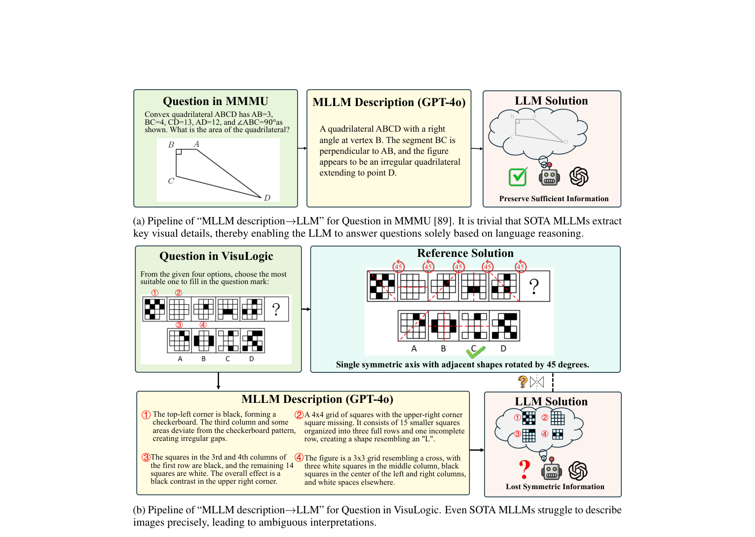Figure 1: VisuLogic shows that VLMs extracting text descriptions from images can answer some benchmarks, but fail on tasks requiring genuine visual reasoning. Source: Xu et al., 2025

The xLogo visual programming benchmark demonstrates this gap concretely. GPT-4V achieves only 20% and Llama3-70B 2.35% on tasks "designed for students up to 2nd grade, where humans can successfully solve almost all tasks" (Wen et al., 2024). You cannot write SVG code that draws a triangle at coordinates (100, 50) to (200, 150) to (50, 150) without understanding coordinate geometry. You cannot write a Blender script placing a red sphere behind a blue cube without understanding depth and occlusion. The models that ace MMLU cannot draw a triangle in the right place.

The RL framing turns this gap into a training signal: the environment tells the model how far off its rendering is, not just whether it passed or failed.

Environment 1: SVG Round-Trip Vectorization

The simplest version of this idea: show the model a PNG of a simple shape, have it output SVG code, render the SVG back to PNG, and score the result.

Pipeline

The pipeline has four stages:

1. Observation: A target PNG (line art, icon, simple geometric composition)
2. Action: The model generates SVG XML as a text string
3. Rendering: cairosvg converts the SVG to a PNG of identical dimensions
4. Reward: Compare the rendered PNG against the target

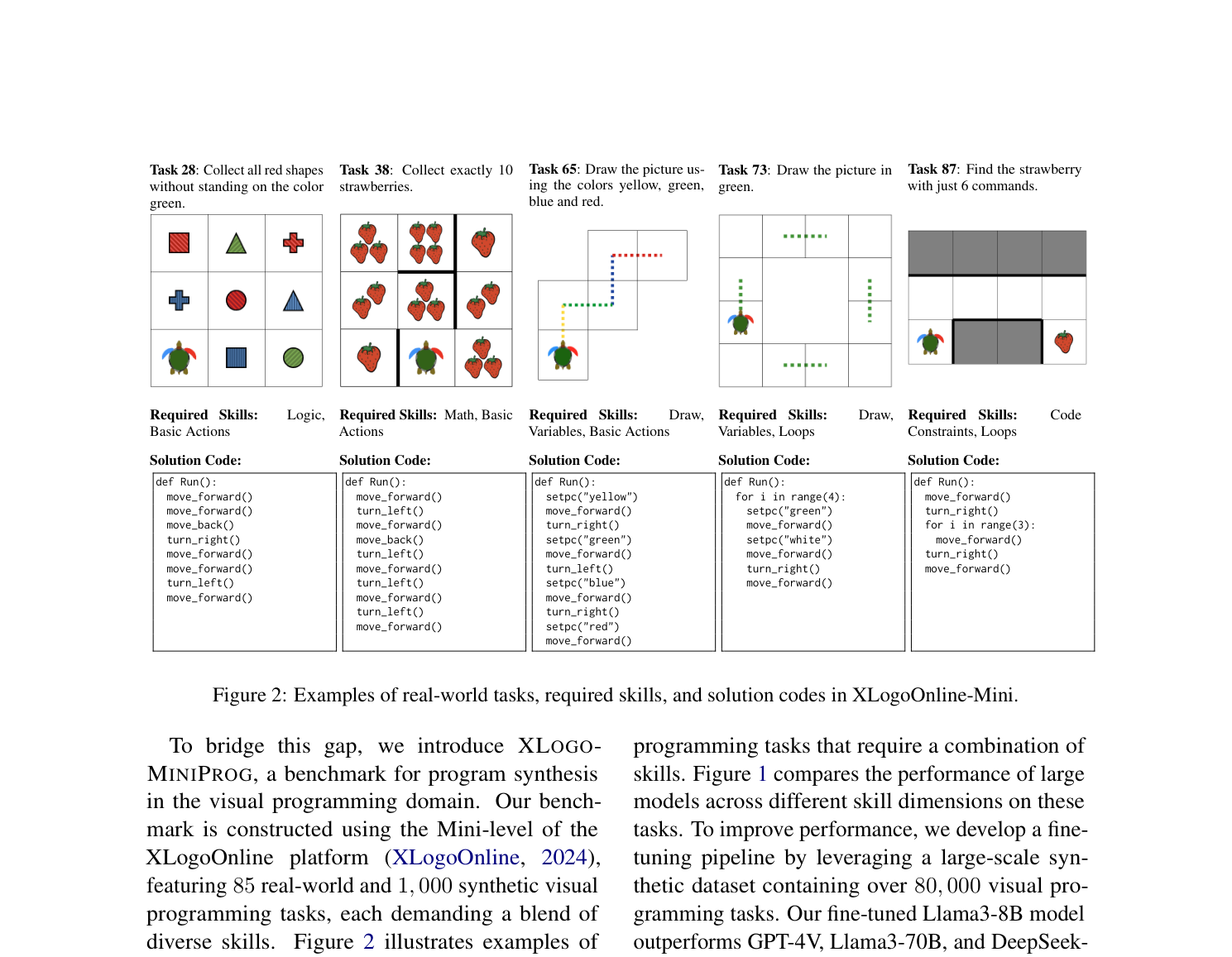Figure 2: xLogo demonstrates the core pattern: visual targets paired with executable code solutions. The same principle applies to SVG generation. Source: Wen et al., 2024

This wraps cleanly into a Gymnasium environment:

import io, xml.etree.ElementTree as ET
import gymnasium as gym
from gymnasium import spaces
import numpy as np
import cairosvg
from PIL import Image

IMG_SIZE = 64  # render resolution (64x64 RGB)


class InverseSVGEnv(gym.Env):
    """Single-step RL env: observe a target PNG, act with an SVG string."""

    metadata = {"render_modes": []}

    def __init__(self, target_images: list[np.ndarray] | None = None):
        super().__init__()
        # Fall back to random white-noise targets for quick testing
        self.targets = target_images or [
            np.random.randint(0, 255, (IMG_SIZE, IMG_SIZE, 3), dtype=np.uint8)
            for _ in range(16)
        ]
        self.observation_space = spaces.Box(
            0, 255, shape=(IMG_SIZE, IMG_SIZE, 3), dtype=np.uint8
        )
        self.action_space = spaces.Text(min_length=1, max_length=4096)
        self.target = self.targets[0]

    def reset(self, *, seed=None, options=None):
        super().reset(seed=seed)
        idx = self.np_random.integers(len(self.targets))
        self.target = self.targets[idx]
        return self.target.copy(), {}

    def step(self, svg_string: str):
        try:
            ET.fromstring(svg_string)  # validate XML
            png_bytes = cairosvg.svg2png(
                bytestring=svg_string.encode(), output_width=IMG_SIZE,
                output_height=IMG_SIZE,
            )
            rendered = np.array(Image.open(io.BytesIO(png_bytes)).convert("RGB"))
        except Exception:
            # Malformed SVG: zero reward, episode over
            return self.target.copy(), 0.0, True, False, {"rendered": None}

        mse = float(np.mean((self.target.astype(np.float32)
                             - rendered.astype(np.float32)) ** 2))
        reward = 1.0 - mse / 65025.0  # normalise by 255^2
        return self.target.copy(), reward, True, False, {"rendered": rendered}

Dataset Selection

For training data, you want controlled complexity. Start with procedurally generated shapes (circles, rectangles, polygons with known SVG representations) before scaling to real-world icons. QuickDraw provides 70K training samples per class with 2.5K validation and 2.5K test samples (Ha and Eck, 2018), though its stroke-based format needs rasterization first. FontAwesome icons offer clean, well-structured SVGs at varying complexity levels.

The CLEVR dataset is worth considering for structured 2D projections. It contains "100K rendered images" with scene graphs providing "ground-truth locations, attributes, and relationships" (Johnson et al., CVPR 2017). CLEVR images are "generated by randomly sampling a scene graph and rendering it using Blender" (Johnson et al., 2017), so the ground-truth scene specification already exists. The constrained vocabulary is a feature, not a limitation: three shapes, two sizes, two materials, and eight colors give the agent a bounded problem where the challenge is purely spatial.

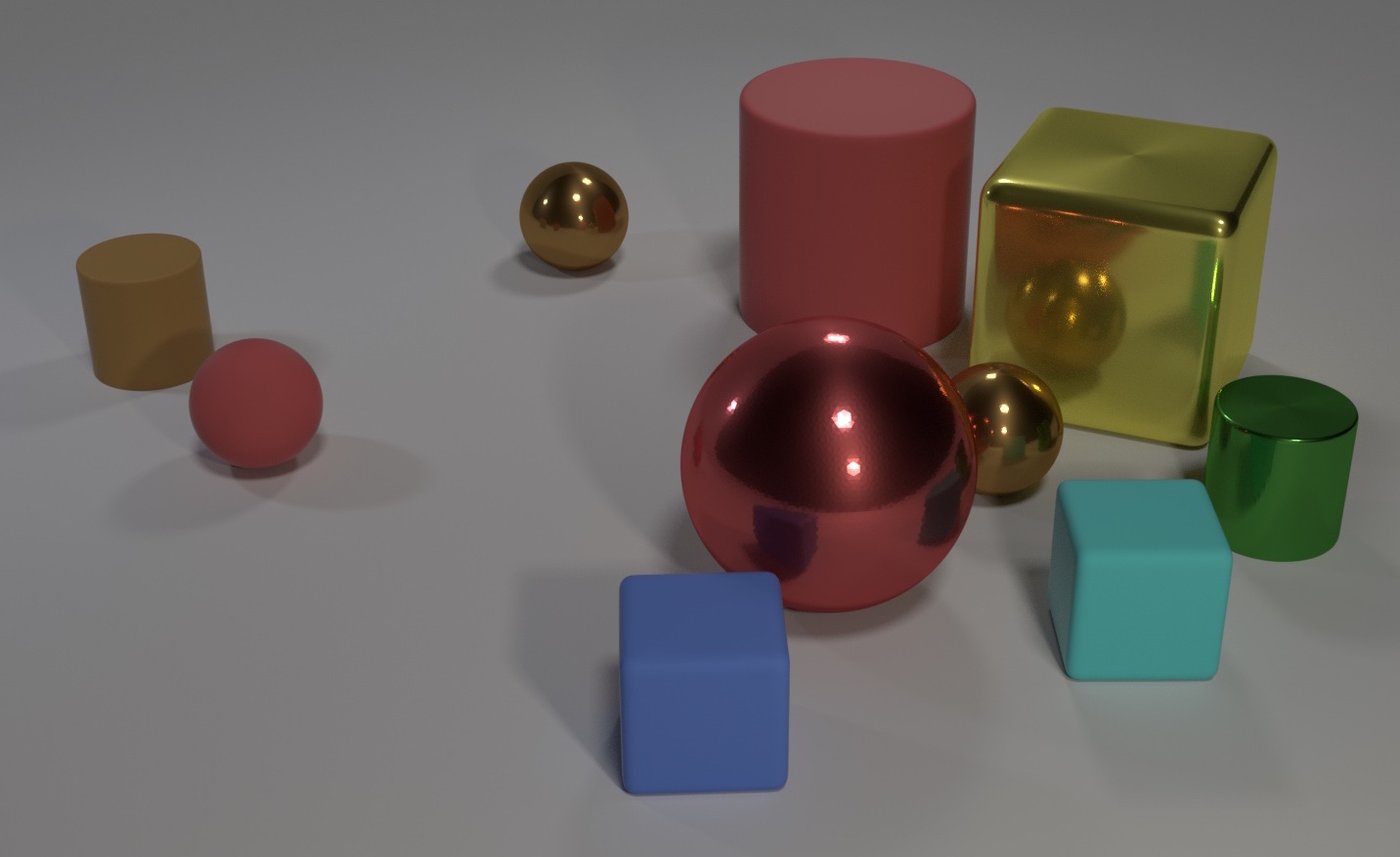Figure 3: CLEVR scenes have known scene graphs with exact object positions, colors, materials, and spatial relationships. Source: Johnson et al., CVPR 2017

Why SVG First

SVG rendering is computationally trivial. cairosvg typically converts SVG to PNG in single-digit milliseconds. This matters for RL, where you need thousands of episodes to see meaningful policy improvement. The action space (text) maps directly to what language models already generate. And the failure mode (malformed XML) is easy to detect and penalize without running the full render pipeline.

The hard part: small SVG syntax errors (a missing closing tag, an unclosed path) produce zero output. This creates sparse rewards. You need either a syntax-checking wrapper that provides partial credit for valid-but-wrong SVG, or a multi-step formulation where the model can iterate on its output.

Environment 2: 3D Scene Reconstruction via Blender

The 3D version is harder across every dimension, but tests deeper spatial understanding: depth, occlusion, lighting, material properties, and perspective projection.

Pipeline

The structure mirrors the SVG environment but substitutes Blender's Python API (bpy) for cairosvg:

1. Observation: A rendered image of a 3D scene
2. Action: A Python script using the bpy API to construct geometry, set materials, position camera and lights
3. Rendering: Blender executes the script headlessly and renders to PNG
4. Reward: Compare rendered output against target

What Makes 3D Harder

Three factors make 3D reconstruction substantially more difficult than 2D vectorization.

Rendering latency. Here is where the engineering gets painful. A headless Blender render takes seconds to minutes depending on scene complexity, compared to milliseconds for SVG. Using Blender's EEVEE engine instead of Cycles gets you to roughly 200ms per render, or about 5 episodes per second per GPU. That remains orders of magnitude slower than SVG. Batching renders across GPUs increases throughput, and proxy reward models can bypass Blender for most training steps, but the computational cost per step remains high.

Camera alignment. Even if the model reconstructs the correct 3D scene, a small camera position error produces large pixel differences. This is why pixel-wise metrics fail for 3D evaluation; you need perceptual metrics (LPIPS, CLIP) that tolerate small viewpoint shifts. One practical fix: lock the camera and lighting in the environment specification, providing the exact camera parameters as part of the observation. The agent's job becomes reconstructing the scene in a known coordinate frame.

Action space complexity. A Blender script can specify meshes, materials, modifiers, particle systems, and more. Constraining the action space is essential. Starting with CLEVR's universe, "three object shapes (cube, sphere, and cylinder) that come in two absolute sizes (small and large), two materials (shiny metal and matte rubber), and eight colors" with "between three and ten objects" per scene (Johnson et al., 2017). This keeps the problem tractable while still testing genuine 3D reasoning.

Tradeoffs: SVG vs. Blender

Dimension	SVG Round-Trip	Blender 3D
Render time per step	~5ms	~200ms-30s
Action space complexity	2D coordinates, paths	3D positions, rotations, materials, lights
Reward signal clarity	High (2D alignment)	Lower (viewpoint-dependent)
Spatial reasoning depth	Moderate (2D composition)	High (3D geometry, occlusion, depth)
Infrastructure cost	Minimal (cairosvg)	Heavy (Blender headless)
Dataset availability	QuickDraw, icons, procedural	CLEVR, Objaverse

The recommendation: build the SVG environment first. It gives a fast, reliable sandbox to iterate on reward functions, agent architectures, and training infrastructure before taking on the Blender overhead.

Reward Design: The Core Engineering Challenge

The choice of reward function determines what the agent actually learns. Build the reward function first; everything else depends on it.

Metric	Speed	Geometric Precision	Perceptual Quality	Viewpoint Invariance
Pixel MSE	Fast	High (brittle)	Low	None
IoU	Fast	Medium	Low	None
SSIM	Fast	Medium	Medium	Low
LPIPS	Medium	Medium	High	Low
CLIP	Slow	Low	Medium	Medium
Composite	Medium	Tunable	Tunable	Tunable

Pixel-wise MSE/IoU: Fast to compute, easy to understand. But brittle. An SVG circle shifted 3 pixels right produces the correct shape with a terrible pixel score.

LPIPS (Learned Perceptual Image Patch Similarity): Uses deep features from a pretrained network to compare perceptual similarity rather than raw pixels. More forgiving of minor positional offsets while still penalizing structural errors.

CLIP embedding distance: Compares images in CLIP's semantic space. Useful for judging overall composition, but too coarse for geometric precision.

For the SVG environment, a composite reward works well: 0.6 * LPIPS + 0.2 * SSIM + 0.2 * pixel_IoU. For 3D scenes, weight LPIPS higher and add a syntax validity bonus (did the Blender script parse and execute at all?).

import numpy as np
import torch
import lpips
from PIL import Image
from skimage.metrics import structural_similarity as ssim

# Initialise LPIPS once (AlexNet backbone, lightweight and fast)
_lpips_fn = lpips.LPIPS(net="alex", verbose=False)


def compute_reward(
    target: Image.Image,
    rendered: Image.Image,
    syntax_valid: bool = True,
    syntax_bonus: float = 0.1,
) -> float:
    """Return a reward in roughly [0, 1+syntax_bonus].

    Components (all mapped so higher = better):
      - 0.6 * (1 - LPIPS)   perceptual similarity
      - 0.2 * SSIM           structural similarity
      - 0.2 * (1 - MSE)      pixel accuracy
      + syntax_bonus          if the source code parsed without errors
    """
    size = (64, 64)
    tgt = np.asarray(target.resize(size).convert("RGB"), dtype=np.float32)
    ren = np.asarray(rendered.resize(size).convert("RGB"), dtype=np.float32)

    # Normalised MSE (0 = identical, 1 = max divergence)
    mse_norm = float(np.mean((tgt - ren) ** 2)) / 65025.0  # 255^2

    # LPIPS (lower = more similar)
    def _to_tensor(arr):
        return torch.from_numpy(arr / 127.5 - 1.0).permute(2, 0, 1).unsqueeze(0).float()

    with torch.no_grad():
        lpips_dist = float(_lpips_fn(_to_tensor(tgt), _to_tensor(ren)))

    # SSIM (higher = more similar)
    ssim_score = float(ssim(tgt, ren, channel_axis=2, data_range=255.0))

    reward = (0.6 * (1.0 - lpips_dist)
              + 0.2 * ssim_score
              + 0.2 * (1.0 - mse_norm)
              + syntax_bonus * float(syntax_valid))
    return reward

Figure 4: PXPO demonstrates that pixel-level reward signals (per-region feedback heatmaps) produce faster convergence than scalar rewards. The same principle applies to inverse graphics: tell the agent where its rendering is wrong, not just how wrong it is. Source: Kordzanganeh et al., 2024

Recent work validates this approach. The PXPO algorithm extends DDPO by providing a per-pixel reward heatmap rather than a scalar, giving "a more nuanced reward to the model" (Kordzanganeh et al., 2024). And the Pixel Reasoner work shows that RL with visual rewards is viable but requires careful warm-starting: pure RL creates "a learning trap that impedes the effective acquisition of pixel-space reasoning" (Wang et al., 2025). Supervised fine-tuning on (image, code) pairs before switching to RL avoids this collapse.

Figure 5: Pixel Reasoner combines supervised warm-start with curiosity-driven RL, overcoming the learning trap in pixel-space reasoning. Their 7B model achieves 84% on V*bench, outperforming proprietary models. Source: Wang et al., 2025

What This Tests That Benchmarks Do Not

Standard VLM benchmarks measure recognition. Inverse graphics environments measure reconstruction. The difference matters:

• Coordinate precision: Placing objects at exact positions, not "roughly left of center"
• Compositional structure: Understanding how shapes relate spatially, not just what they are
• Symbolic grounding: Translating visual understanding into executable code
• Iterative refinement: Using feedback to improve, not just producing one-shot answers

The xLogo benchmark showed that fine-tuning a Llama3-8B model on 80K synthetic tasks boosted it to 54.12% success, outperforming GPT-4V (20%) and even DeepSeek-R1-Distill (44.71%) (Wen et al., 2024). That gap between zero-shot and fine-tuned performance is exactly the opportunity space for RL.

The VisuLogic authors demonstrated this directly: "a simple reinforcement-learning fine-tuning step on our supplementary training dataset boosted the baseline model's accuracy from 25.5% to 31.1%, outperforming both open-source and closed-source counterparts" (Xu et al., 2025). RL works for visual reasoning. Inverse graphics gives it a richer, more structured reward surface.

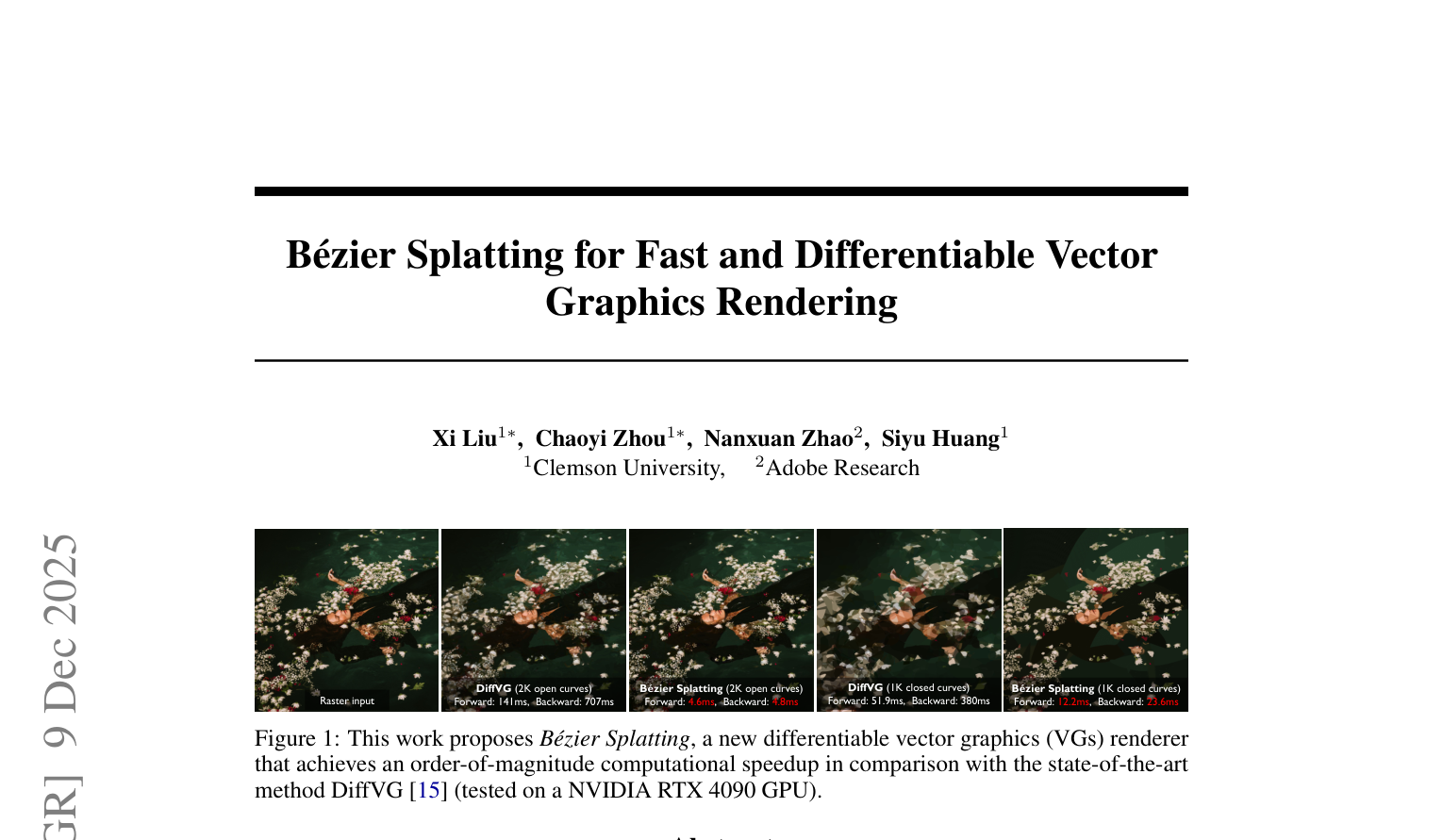Figure 6: Bezier Splatting achieves 30x forward and 150x backward speedup over DiffVG for differentiable vector graphics rendering (4.6ms vs. 141ms forward on 2K open curves). This opens the door to hybrid approaches: differentiable rendering for coarse optimization, then code-based RL for structured output. Source: Liu et al., 2025

Practical Roadmap

If you want to build this, here is a concrete timeline:

Week 1: Build the Gymnasium wrapper. Use cairosvg for rendering, SSIM for initial rewards. Generate a dataset of 1,000 procedural SVGs (random circles, rectangles, basic compositions with known ground-truth SVG).

Week 2: Add LPIPS rewards and the composite metric. Test with a pretrained VLM (GPT-4o, Claude, Gemini) in a zero-shot setting to establish baselines. Expect low initial success rates; the xLogo results suggest frontier models achieve 20-44% on much simpler visual programming tasks (Wen et al., 2024).

Week 3: Implement multi-turn refinement. Let the model see its own render alongside the target and iterate. This is where RL becomes useful: the agent learns not just to generate code but to debug it. Track three metrics separately: valid SVG rate, structural match (SSIM > 0.8), and geometric precision (LPIPS < 0.1).

Month 2: Scale to CLEVR-style scenes and consider the Blender environment. The SynthRL approach of synthesizing training data with verified difficulty (Wu et al., 2025) maps directly: generate scenes of increasing complexity, verify that each is solvable, and use the difficulty gradient as a curriculum.

Limitations

This approach tests spatial code generation specifically, not general spatial understanding. A model that excels at SVG reconstruction may still fail at navigation, mental rotation, or spatial relationship reasoning. The SVG environment also biases toward 2D geometry; 3D spatial reasoning requires the Blender environment with its latency costs.

The reward design problem is not fully solved. LPIPS and CLIP are proxies for visual similarity, not ground-truth metrics. A compositionally correct scene rendered with slightly different line weights could score poorly despite being semantically perfect. And the action space (raw code) may be too unconstrained for efficient RL exploration; structured action spaces trading expressiveness for tractable exploration remain worth investigating.

Conclusion

VLMs claim spatial understanding. Inverse graphics RL environments call that bluff. By requiring models to produce executable code that renders to match a target image, these environments test coordinate precision, compositional structure, and symbolic grounding in ways that multiple-choice benchmarks cannot.

The SVG round-trip environment is buildable today with off-the-shelf tools: Gymnasium, cairosvg, LPIPS. The 3D Blender environment is harder but tests deeper spatial reasoning. Both provide verifiable, continuous reward signals suitable for RL training. The evidence from recent work, including Pixel Reasoner, SynthRL, and VisuLogic, confirms that RL with visual rewards improves spatial reasoning. The verifier is a renderer, and renderers do not have opinions.

---

References

• Xu et al., "VisuLogic: A Benchmark for Evaluating Visual Reasoning in Multi-modal Large Language Models," 2025. arXiv:2504.15279

• Ha and Eck, "A Neural Representation of Sketch Drawings," ICLR 2018. arXiv:1704.03477

• Wen et al., "Program Synthesis Benchmark for Visual Programming in XLogoOnline Environment," 2024. arXiv:2406.11334

• Johnson et al., "CLEVR: A Diagnostic Dataset for Compositional Language and Elementary Visual Reasoning," CVPR 2017. arXiv:1612.06890

• Kordzanganeh et al., "Pixel-wise RL on Diffusion Models: Reinforcement Learning from Rich Feedback," 2024. arXiv:2404.04356

• Wang et al., "Pixel Reasoner: Incentivizing Pixel-Space Reasoning with Curiosity-Driven Reinforcement Learning," 2025. arXiv:2505.15966

• Wu et al., "SynthRL: Scaling Visual Reasoning with Verifiable Data Synthesis," 2025. arXiv:2506.02096

• Liu et al., "Bezier Splatting for Fast and Differentiable Vector Graphics Rendering," 2025. arXiv:2503.16424