End-to-End Test-Time Training: Making Long Context Work Without the Memory Tax

Despite LLMs now supporting 128K context windows, users still copy-paste earlier context back into the chat. The model forgets mid-conversation details that a human would retain effortlessly. This is not a minor UX annoyance. It represents a fundamental tension in how we build language models: the quadratic cost of attention makes long context prohibitively expensive, yet every workaround trades away some portion of the model's ability to reason over the full context.

What if we reframed the problem entirely? Instead of treating long context as an architecture challenge requiring ever-more-efficient attention mechanisms, what if we treated it as a learning problem where the model compresses context into its weights during inference?

This is the core insight behind End-to-End Test-Time Training (TTT-E2E). The approach "formulate[s] long-context language modeling as a problem in continual learning rather than architecture design."¹ Rather than storing all context in a KV cache or retrieving relevant chunks, TTT-E2E has the model learn from its context in real-time, compressing information into weight updates that persist through the sequence.

The results speak for themselves: constant inference latency regardless of context length, "2.7x faster than full attention for 128K context,"² and scaling behavior that matches full-attention transformers while maintaining the efficiency of linear-complexity architectures.

Table of Contents

• The Long Context Problem
• How Test-Time Training Works
• The End-to-End Formulation
• Architecture and Implementation
• Benchmark Results
• Comparison with Alternatives
• When to Use TTT-E2E
• Limitations and Future Directions
• Conclusion

The Long Context Problem

Standard transformer attention has a fundamental scaling problem. "Self-attention over the full context, also known as full attention, must scan through the keys and values of all previous tokens for every new token."³ This translates to computational complexity of "O(T^2) for prefill and O(T) for decode"⁴ where T is the context length.

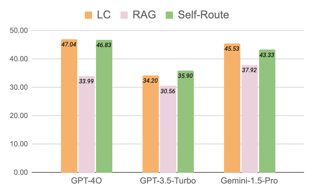Figure 1: Different approaches to handling large amounts of information in LLMs. Source: Liu et al. (2024)

For a 128K context window, this means approximately 16 billion attention computations just for the prefill phase. Even with FlashAttention's memory optimizations, which "reduce[s] the number of memory reads/writes between GPU high bandwidth memory (HBM) and GPU on-chip SRAM"⁵ and achieves "up to 7.6x speedup on GPT-2"⁶, the fundamental compute cost remains quadratic.

The alternatives each come with tradeoffs:

RAG (Retrieval-Augmented Generation): Retrieves relevant chunks rather than processing full context. Cost-effective but misses cross-document reasoning and adds retrieval latency.

Sliding Window Attention: Limits attention to recent tokens. Linear complexity but loses access to earlier context entirely.

State Space Models (Mamba): "Mamba enjoys fast inference (5x higher throughput than Transformers) and linear scaling in sequence length."⁷ But current SSMs still underperform transformers on tasks requiring precise information retrieval from long context, due to their "inability to perform content-based reasoning."⁸

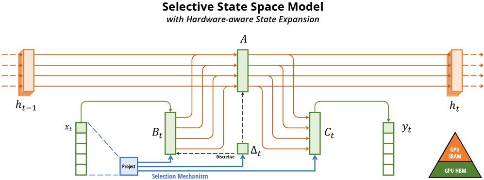Figure 2: Mamba's selective state space architecture enables linear-time sequence modeling by making state transitions input-dependent. Source: Gu & Dao (2023)

The fundamental issue is that all these approaches treat context as data to be stored, cached, or retrieved. TTT takes a different view: context is training signal.

How Test-Time Training Works

The key insight is deceptively simple: "our model continues learning at test time via next-token prediction on the given context, compressing the context it reads into its weights."⁹

Instead of storing context in a KV cache, TTT updates a subset of the model's weights as it processes each token. The model studies the context, learning patterns and facts that it can then use for generation.

This is not fine-tuning. Fine-tuning happens before deployment. TTT happens during inference, on the specific context the model is processing. Each sequence gets its own temporary weight updates that compress the relevant information.

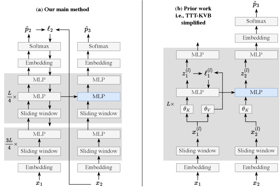Figure 3: TTT-E2E architecture comparison. Left: Prior TTT approaches required separate pretraining. Right: TTT-E2E meta-learns the initialization, treating training sequences as test sequences in the inner loop. Source: Sun et al. (2025)

The learning objective is straightforward: next-token prediction on the context itself. "We update W at test time for every t=1,...,T, in sequential order, with gradient descent."¹⁰ As the model reads each token, it:

1. Makes a prediction for the next token
2. Observes the actual next token
3. Updates its weights to reduce prediction error
4. Moves to the next position with updated weights

This creates a form of online learning where the model continuously adapts to the specific patterns in the current context.

The complexity analysis reveals why this matters:

Operation	Full Attention	TTT
Prefill	O(T^2)	O(T)
Decode	O(T)	O(1)

"Test-Time Training (TTT) has O(T) for prefill and O(1) for decode."¹¹ That O(1) decode complexity is the key advantage: inference latency becomes constant regardless of how long the context is.

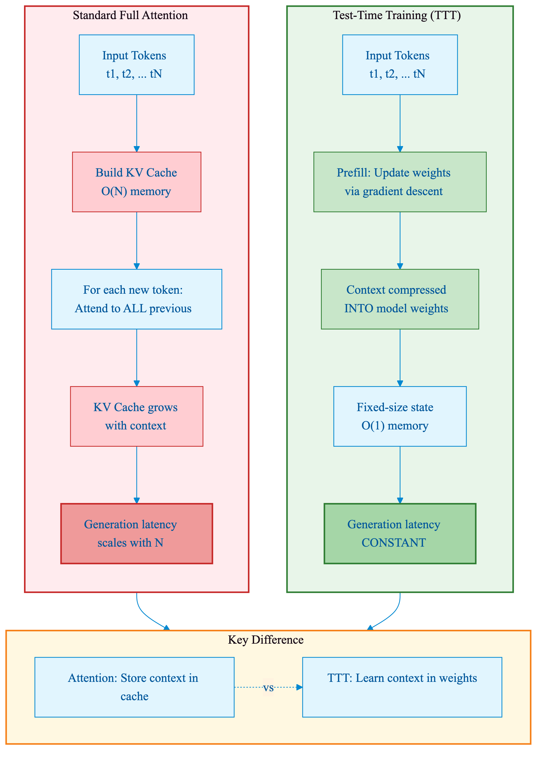Figure 3a: Side-by-side comparison of Standard Full Attention (left) with growing KV cache versus TTT (right) with weight updates. TTT compresses context into weights rather than storing it in cache, achieving constant-time generation.

The End-to-End Formulation

Previous TTT approaches trained the model in two separate phases: first conventional pretraining, then adapting a test-time learning procedure on top. TTT-E2E unifies these through meta-learning.

"We improve the model's initialization for learning at test time via meta-learning at training time."¹²

The training procedure works in two nested loops:

Inner Loop (Test-Time Training): "Each training sequence is first treated as if it were a test sequence, so we perform TTT on it in the inner loop."¹³ The model processes the sequence token-by-token, updating weights via gradient descent on next-token prediction.

Outer Loop (Meta-Learning): The outer loop optimizes the model's initial weights so that the inner-loop learning produces good final predictions. The outer loss depends on the model's performance after the inner loop has run.

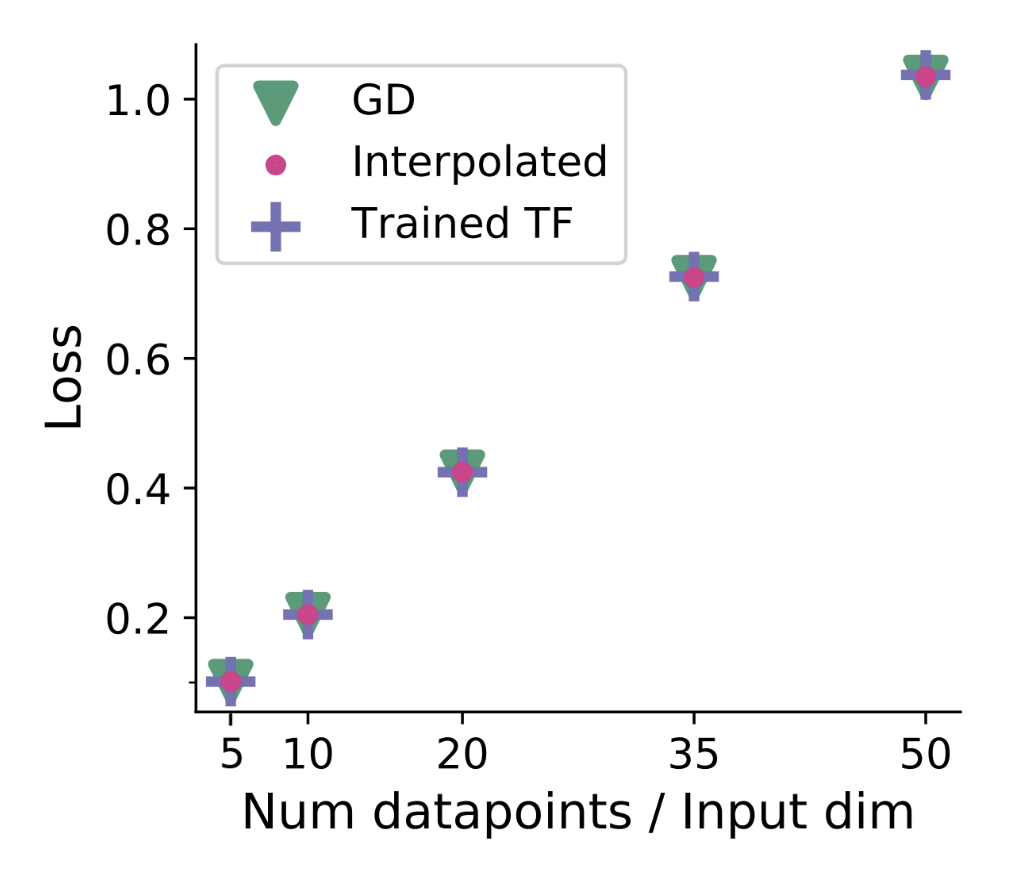Figure 4: Transformers implement implicit gradient descent during in-context learning. TTT makes this optimization explicit. Source: Von Oswald et al. (2023)

The theoretical basis comes from work showing that "when training Transformers on auto-regressive tasks, in-context learning in the Transformer forward pass is implemented by gradient-based optimization."¹⁴ TTT-E2E makes this implicit optimization explicit, running actual gradient descent rather than relying on attention to simulate it.

This meta-learning formulation has biological motivation. "Considering that infants rapidly accumulate knowledge with minimal forgetting, it seems plausible that humans have likely developed their capacity for continual and online learning through the process of biological evolution rather than solely within an individual's lifetime."¹⁵ TTT-E2E optimizes the learning algorithm itself, not just the learned knowledge.

def inner_loop_ttt(sequence, initial_weights, learning_rate, mini_batch_size):
    """
    Inner loop: Perform Test-Time Training on a single sequence.

    For mini-batch TTT:
        W_i = W_{i-1} - eta * (1/b) * sum(gradient(loss_t(W_{i-1})))
    """
    current_weights = initial_weights.copy()
    all_losses = []

    for batch_idx in range(len(sequence) // mini_batch_size):
        accumulated_gradient = {}

        for t in range(batch_idx * mini_batch_size, (batch_idx + 1) * mini_batch_size):
            # Compute loss for predicting x_t from x_{t-1}
            loss_t = compute_next_token_loss(current_weights, sequence[t-1], sequence[t])
            all_losses.append(loss_t)

            # Accumulate gradients over mini-batch
            grad_t = compute_gradient(loss_t, current_weights)
            for key in grad_t:
                accumulated_gradient[key] = accumulated_gradient.get(key, 0) + grad_t[key]

        # Gradient descent: W_i = W_{i-1} - eta * grad
        for key in current_weights:
            current_weights[key] -= learning_rate * accumulated_gradient[key] / mini_batch_size

    return current_weights, all_losses


def outer_loop_meta_learning(training_sequences, W_0, outer_lr, inner_lr, mini_batch_size):
    """
    Outer loop: Meta-learning to optimize initial weights for TTT.

    CRITICAL: Gradients must flow through the inner loop!
    We compute d(L)/d(W_0), which requires differentiating through
    the inner loop gradient descent steps.
    """
    for sequence in training_sequences:
        # Inner loop: treat training sequence as test
        final_weights, losses = inner_loop_ttt(sequence, W_0, inner_lr, mini_batch_size)

        # Outer loss depends on W_0 through the inner loop
        sequence_loss = sum(losses) / len(losses)

        # Compute gradient through inner loop (gradients of gradients)
        # Modern autograd handles this efficiently
        grad_outer = compute_gradient(sequence_loss, W_0)

        # Update initial weights
        W_0 = {k: W_0[k] - outer_lr * grad_outer[k] for k in W_0}

    return W_0  # Optimized for test-time learning

Code 1: TTT-E2E training loop pseudocode showing nested optimization. The inner loop simulates test-time training; the outer loop optimizes initial weights so inner-loop learning produces good predictions.

The key engineering insight is that "modern frameworks for automatic differentiation can efficiently compute gradients of gradients with minimal overhead."¹⁶ This makes the bilevel optimization tractable, though training is approximately 3.4x slower than standard pretraining.

Architecture and Implementation

Converting a standard transformer to TTT-E2E requires careful architectural decisions. Not all parameters should be updated during test-time training.

Which Layers to Update: Not all layers benefit equally from test-time adaptation. "We choose to TTT only the last 1/4 of the blocks according to the ablations."¹⁷ Earlier layers learn more general features that transfer well; later layers learn more context-specific patterns that benefit from adaptation.

Stability Mechanisms: "We freeze the embedding layers, normalization layers, and attention layers during TTT, since updating them in the inner loop causes instability in the outer loop."¹⁸ Only the MLP weights receive gradient updates at test time.

Preserving Pretrained Knowledge: A key concern with any weight update is catastrophic forgetting. "Training a neural network naively on such a non-stationary stream using stochastic gradient descent (SGD) consistently overwrites the knowledge of the previous tasks, which is referred to as catastrophic forgetting."¹⁹

TTT-E2E addresses this directly: "In the blocks updated during TTT, we add a static, second MLP layer as a safe storage for pre-trained knowledge."²⁰ This dual-MLP design separates context-specific adaptations from permanent knowledge. The original MLP preserves general capabilities while the new MLP learns context-specific patterns.

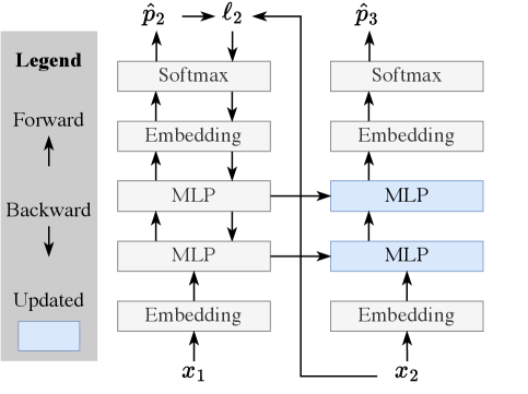Figure 5: TTT layer architecture showing MLP weight updates during forward pass. The inner model learns from context through next-token prediction, compressing information into weight updates. Source: Sun et al. (2025)

Hyperparameters: "For our main results with T = 128K, we set the window size k to 8K and the TTT mini-batch size b to 1K."²¹ The window size determines how much context is used for each gradient update; the mini-batch size controls the granularity of weight updates.

Integration with Sliding Window: TTT layers work effectively with sliding window attention for practical deployment. "TTT layers can effectively use inner-loop mini-batch gradient descent when preceded by sliding-window attention layers."²² The attention handles local patterns within the window while TTT captures long-range dependencies through accumulated weight updates.

from dataclasses import dataclass, field

@dataclass
class TTTHyperparameters:
    """From paper: 'For T=128K, we set window size k to 8K and mini-batch size b to 1K.'"""
    max_context_length: int = 128_000  # T = 128K tokens
    sliding_window_size: int = 8_000   # k = 8K (attention window)
    ttt_mini_batch_size: int = 1_000   # b = 1K (gradient update frequency)
    ttt_block_fraction: float = 0.25   # Final 1/4 of blocks

@dataclass
class TTTModelConfig:
    """Configuration for TTT-E2E enabled transformer."""
    num_layers: int = 24
    hidden_dim: int = 1536
    ttt_params: TTTHyperparameters = field(default_factory=TTTHyperparameters)

    def get_frozen_layers(self) -> list:
        """Layers frozen during TTT to prevent instability."""
        return ["embedding", "normalization", "attention"]  # All blocks

    def get_trainable_layers(self) -> list:
        """Only MLP layers in final 1/4 of blocks are trainable."""
        ttt_start = int(self.num_layers * (1 - self.ttt_params.ttt_block_fraction))
        return [f"blocks.{i}.mlp" for i in range(ttt_start, self.num_layers)]

    def has_dual_mlp(self, block_idx: int) -> bool:
        """Dual MLP in TTT blocks: trainable MLP + static MLP for knowledge preservation."""
        ttt_start = int(self.num_layers * (1 - self.ttt_params.ttt_block_fraction))
        return block_idx >= ttt_start

# Example: 3B model with 128K context
config = TTTModelConfig(num_layers=32, hidden_dim=2560)
print(f"TTT-enabled blocks: {config.get_trainable_layers()[-8:]}")  # Final 8 of 32

Code 2: PyTorch-style TTT configuration. Key decisions: freeze attention/norm layers, only update final 1/4 of blocks, add dual-MLP architecture for knowledge preservation.

Connection to Linear Attention: Interestingly, "linear attention and many of its variants, such as Gated DeltaNet, can also be derived from this perspective."²³ TTT provides a unifying framework where different architectures emerge as special cases of test-time learning with different update rules and objectives.

Benchmark Results

TTT-E2E was evaluated across five model sizes. "We experiment with models of five sizes, ranging from 125M to 3B parameters."²⁴ All models were trained on 164B tokens with fine-tuning on "Books, a standard academic dataset for long-context extension."²⁵

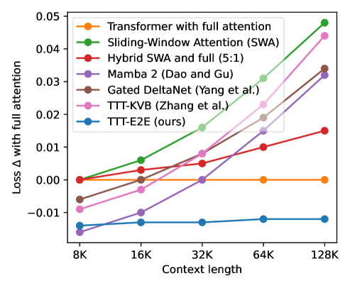Figure 6: Test loss vs context length. TTT-E2E (red) scales with context length in the same way as Transformers with full attention (blue), outperforming Mamba (orange) at 128K context. Source: Sun et al. (2025)

Scaling with Context Length: "For 3B models trained with 164B tokens, our method (TTT-E2E) scales with context length in the same way as Transformer with full attention."²⁶ This is significant because it means TTT-E2E captures the quality benefits of full attention while maintaining efficient complexity.

Latency Advantage: "TTT-E2E has constant inference latency regardless of context length, making it 2.7x faster than full attention for 128K context."² The speedup grows with context length as full attention's latency increases linearly while TTT-E2E remains constant.

Hidden State Efficiency: "Our final method (TTT-E2E), which removes both differences together, has 5x larger hidden state (88M vs. 18M for the 760M model) and half the inference latency (0.0086 vs. 0.017 sec per 1K tokens for prefill on H100)."²⁷ The 5x larger hidden state stores accumulated context-adapted parameters, but this is a fixed cost independent of context length.

Complementarity with Full Attention: Perhaps surprisingly, "TTT-E2E can improve test loss by 0.018 even on top of full attention."²⁸ This suggests TTT-E2E learns something complementary to what attention captures, rather than simply approximating it.

Sliding Window Transformation: Most dramatically: "TTT-E2E turns the worst performing sliding window attention into the best performing method at 128K context length."²⁹ Sliding window attention alone loses information beyond the window. With TTT, that information gets compressed into weights instead of being lost.

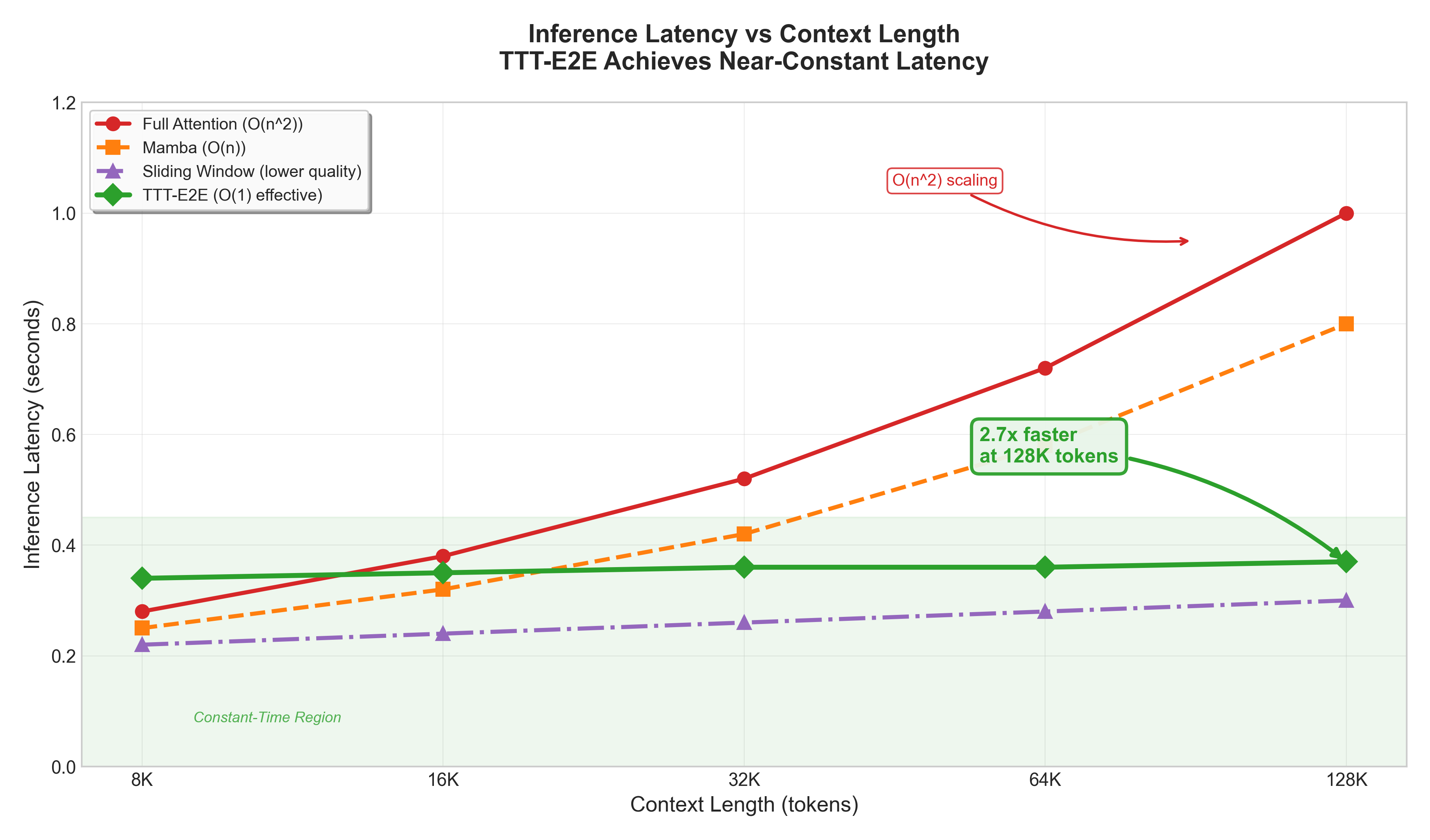Figure 9: Inference latency vs context length. TTT-E2E maintains constant latency regardless of context length, achieving 2.7x speedup over full attention at 128K tokens. Full attention shows quadratic O(n^2) scaling while Mamba scales linearly.

Comparison with Alternatives

How does TTT-E2E compare to other approaches for efficient long context?

vs. Full Attention Transformers

Full attention remains the gold standard for quality on long-context tasks. TTT-E2E matches this quality while providing:

• Constant decode latency (O(1) vs O(T))
• 2.7x speedup at 128K context
• No KV cache memory scaling with context length

The tradeoff: approximately 3.4x slower training due to meta-learning overhead.

vs. Mamba and State Space Models

"On language modeling, our Mamba-3B model outperforms Transformers of the same size and matches Transformers twice its size, both in pretraining and downstream evaluation."³⁰ However, Mamba's selective state mechanism still struggles with precise retrieval from long context compared to attention.

TTT-E2E outperforms Mamba on long-context benchmarks while maintaining comparable inference efficiency:

Method	Prefill	Decode	Quality at 128K
Full Attention	O(T^2)	O(T)	Best
Mamba	O(T)	O(1)	Good
Sliding Window	O(T*k)	O(k)	Poor
TTT-E2E	O(T)	O(1)	Best

Table 1: Complexity comparison of long-context approaches. TTT-E2E achieves quality parity with full attention while matching Mamba's efficiency profile.

vs. FlashAttention

FlashAttention optimizes how attention is computed but does not change its fundamental complexity. "FlashAttention trains Transformers faster than existing baselines: 15% end-to-end wall-clock speedup on BERT-large (seq. length 512) compared to the MLPerf 1.1 training speed record, 3x speedup on GPT-2 (seq. length 1K)."³¹

FlashAttention and TTT are complementary: you can use FlashAttention for the sliding window attention layers in TTT. But FlashAttention alone cannot achieve constant decode latency.

vs. RAG Systems

RAG maintains cost advantages through selective retrieval rather than processing full context. For tasks requiring comprehensive understanding of long documents where retrieval might miss cross-section dependencies, TTT's compression approach may be more appropriate. For targeted question-answering where relevant chunks are clearly identifiable, RAG remains competitive.

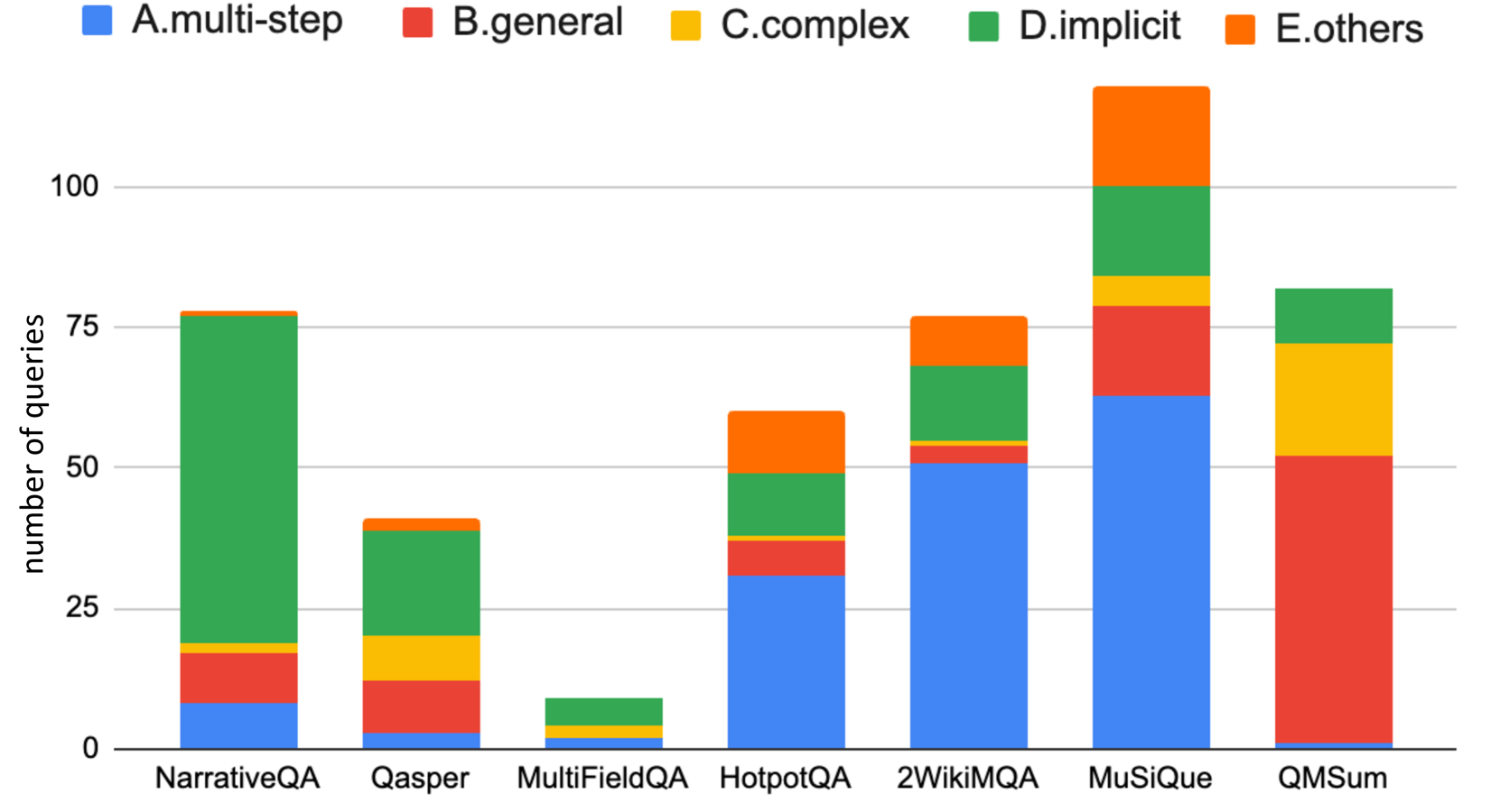Figure 7: Why RAG fails: distribution of failure reasons across datasets. "Not in Context" and "Reasoning Error" dominate, showing retrieval limitations for tasks requiring cross-document reasoning. Source: Liu et al. (2024)

When to Use TTT-E2E

TTT-E2E is not universally optimal. Here is a decision framework based on the research:

Use TTT-E2E when:

• Context length exceeds 64K tokens
• Constant inference latency is required
• The application involves processing long documents repeatedly
• Memory constraints prevent full KV cache storage
• Tasks require reasoning over full context, not just retrieval

Consider alternatives when:

• Context is short (<8K tokens): full attention is simpler and equally fast
• Retrieval suffices: RAG may be more cost-effective for targeted Q&A
• Training compute is severely limited: TTT-E2E training is approximately 3.4x slower
• Real-time streaming is required: TTT has per-token gradient overhead during prefill

Hybrid approaches may work best when:

• Context lengths vary widely across requests
• Some queries need retrieval, others need full reasoning
• Latency budgets allow dynamic routing between approaches

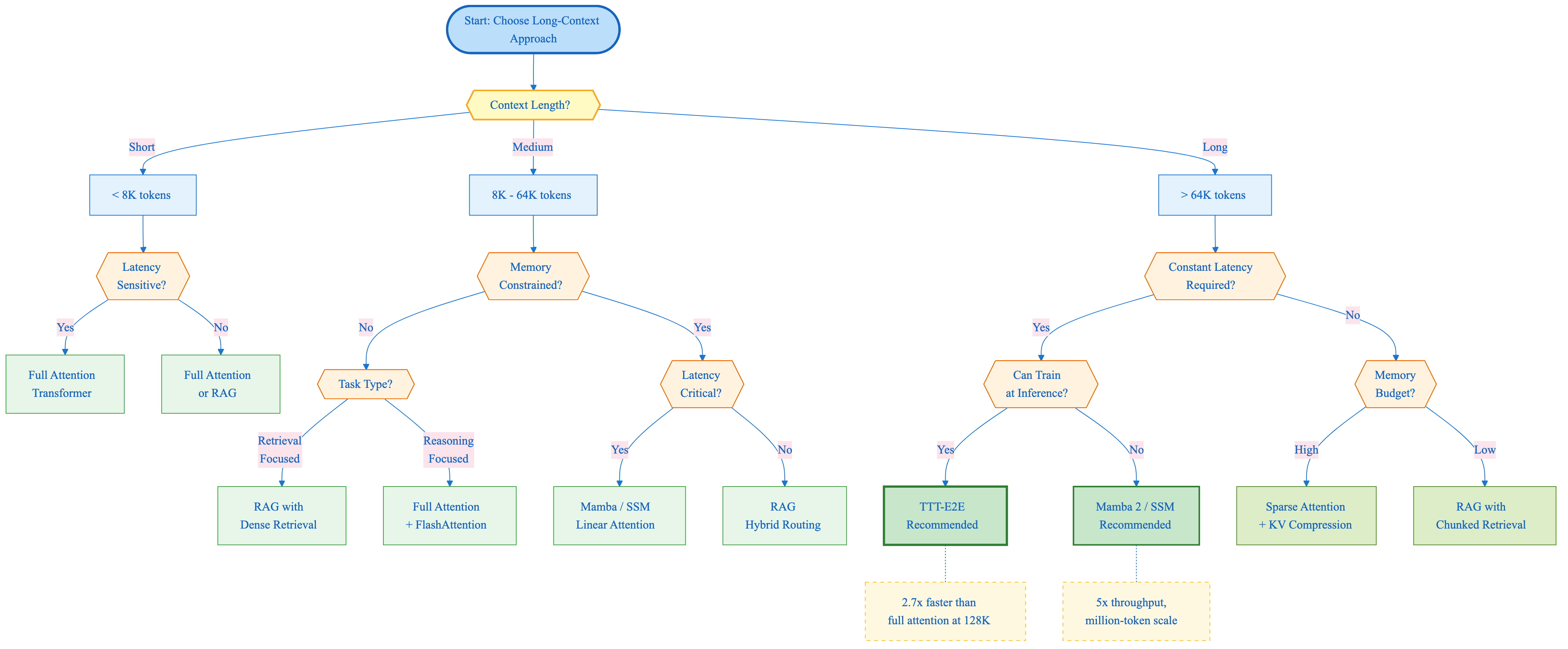Figure 10: Decision tree for choosing between TTT-E2E, Full Attention, RAG, and Mamba based on context length, latency requirements, memory constraints, and task type.

Limitations and Future Directions

Several limitations remain in the current TTT-E2E formulation:

Training Cost: The meta-learning objective requires computing gradients through the inner loop, making training approximately 3.4x slower than standard approaches. For organizations with limited training compute, this overhead may be prohibitive.

Per-Token Gradient Computation: While decode latency is O(1), the prefill phase still requires O(T) for context compression. For real-time streaming applications where immediate response matters, this initial cost is significant.

Context Order Sensitivity: Like other continual learning methods, TTT-E2E's final state depends on the order in which context is processed. Shuffling the same context could yield different results.

Scaling Laws: The paper demonstrates results up to 3B parameters and 128K context. Behavior at larger scales (70B+ parameters, 1M+ context) remains to be characterized.

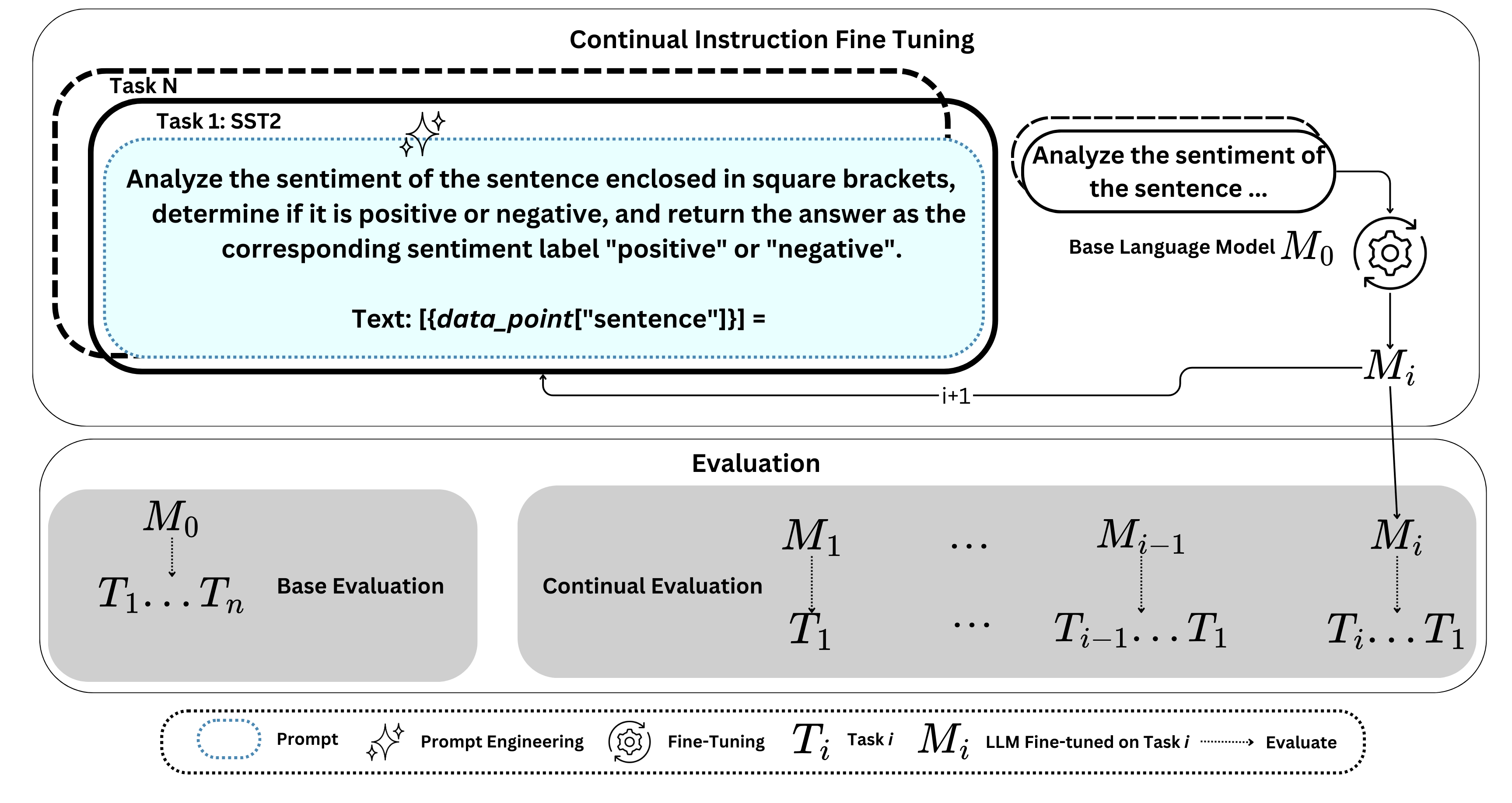Figure 8: Continual instruction fine-tuning workflow illustrating catastrophic forgetting. As models train on sequential tasks (T1...Tn), performance on earlier tasks degrades. TTT avoids this through per-sequence weight updates that don't persist. Source: Yildirim et al. (2025)

Future Directions:

The connection between TTT and in-context learning suggests several research directions. Could selective TTT that identifies which context portions benefit most from compression improve efficiency? Could hybrid architectures combining TTT with Mamba or linear attention provide benefits of both approaches?

"Continual learning remains essential for three key reasons: continual pre-training to keep models up to date, continual fine-tuning for specialization, and continual compositionality for modular intelligence."³² TTT adds a fourth: continual inference-time adaptation for context-specific capabilities.

Conclusion

End-to-End Test-Time Training offers a distinct approach to long context in language models. Rather than fighting the quadratic complexity of attention through architectural innovations, TTT-E2E leans into the learning-based nature of neural networks: if attention is expensive, have the model learn the context instead of storing it.

The practical implications are significant. For applications requiring consistent latency across varying context lengths, whether document analysis, code understanding, or long-form conversation, TTT-E2E provides a path forward that does not sacrifice quality for efficiency.

The key technical innovations are:

1. Context as training signal: Next-token prediction on context compresses information into weights
2. Meta-learned initialization: Training optimizes weights for test-time learning, not just task performance
3. Architectural constraints: Selective layer updates and dual-MLP design prevent catastrophic forgetting

The deeper insight may be that the boundary between training and inference is more fluid than our current frameworks assume. "Each training sequence is first treated as if it were a test sequence"¹³, suggesting that models can and should continue learning throughout their lifecycle, adapting to each new context they encounter.

As context windows continue growing toward document-length and beyond, the question of whether to store or learn from context will only become more pressing. TTT-E2E suggests the answer might be: learn.

---

References

Footnotes

1. Sun et al., "End-to-End Test-Time Training for Long Context," arXiv:2512.23675, December 2025. Lines 10-11. ↩

2. Sun et al. (2025). Lines 20-21. ↩ ↩²

3. Sun et al. (2025). Lines 88-90. ↩

4. Sun et al. (2025). Lines 163-164. ↩

5. Dao et al. (2022). Lines 17-19. ↩

6. Dao et al. (2022). Lines 117-118. ↩

7. Gu & Dao, "Mamba: Linear-Time Sequence Modeling with Selective State Spaces," arXiv:2312.00752, 2023. Lines 18-20. ↩

8. Gu & Dao (2023). Lines 13-16. ↩

9. Sun et al. (2025). Lines 12-13. ↩

10. Sun et al. (2025). Lines 179-180. ↩

11. Sun et al. (2025). Line 165. ↩

12. Sun et al. (2025). Line 14. ↩

13. Sun et al. (2025). Lines 106-108. ↩ ↩²

14. Von Oswald et al., "Transformers Learn In-Context by Gradient Descent," arXiv:2212.07677, 2023. Lines 157-164. ↩

15. Meta-Learning Continual Learning Survey (2023). Lines 377-384. ↩

16. Sun et al. (2025). Lines 234-235. ↩

17. Sun et al. (2025). Lines 298-299. ↩

18. Sun et al. (2025). Lines 291-292. ↩

19. Kirkpatrick et al., referenced in Meta-Learning Continual Learning Survey, arXiv:2311.05241, 2023. Lines 258-261. ↩

20. Sun et al. (2025). Lines 302-304. ↩

21. Sun et al. (2025). Lines 279-280. ↩

22. Sun et al. (2025). Lines 395-396. ↩

23. Sun et al. (2025). Lines 368-369. ↩

24. Sun et al. (2025). Line 502. ↩

25. Sun et al. (2025). Lines 499-501. ↩

26. Sun et al. (2025). Lines 17-19. ↩

27. Sun et al. (2025). Lines 475-478. ↩

28. Sun et al. (2025). Lines 586-587. ↩

29. Sun et al. (2025). Lines 62-63. ↩

30. Gu & Dao (2023). Lines 21-23. ↩

31. Dao et al., "FlashAttention: Fast and Memory-Efficient Exact Attention," arXiv:2205.14135, 2022. Lines 23-25. ↩

32. Wu et al., "The Future of Continual Learning in the Era of Foundation Models," arXiv:2506.03320, 2025. Lines 17-22. ↩